图注意力网络
post on 07 Jun 2020 about 9277words require 31min
CC BY 4.0 (除特别声明或转载文章外)
如果这些文字帮助到你,可以请我喝一杯咖啡~
图卷积网络(Graph Convolutional Network, GCN)告诉我们将局部的图结构和节点特征结合可以在节点分类任务中获得不错的表现;图注意力网络(Graph Attention Network, GAT)则在 GCN 的基础之上引入了注意力机制,从而克服了先前图卷积网络的短板。下面三篇论文有递进关系,这篇笔记着重整理其中第二篇论文:
- Semi-Supervised Classification with Graph Convolutional Networks,ICLR 2017,图卷积网络
- Graph Attention Network,ICLR 2018,图注意力网络
- Relational Graph Attention Networks,ICLR2019,关联性图注意力网络,整合了 GCN+Attention+Relational
方法介绍
针对每一个节点运算相应的隐藏信息,在运算其相邻节点的时候引入注意力机制,有如下几个特性与优势:
- 高效,与 GCN 的复杂度相当,并且可以并行运算。
- 针对有不同度数(degree)的节点,可以运用任意大小的权重与之对应。
- 可用于归纳学习(inductive learning),新来节点的时候,只需要考虑邻居的信息,对 GAT 的影响并不大(使用 GCN 时整个图矩阵就发生了变化,需要重新训练模型)
在四个数据集(Cora、Citeseer、Pubmed、protein interaction)上达到 state of the art 的准确率。
图注意力层(Graph Attention Layer)
输入 $\mathbf{h}$ 为 $N$ 个节点的每个节点的 $F$ 个特征。
\[\mathbf{h}=\lbrace \vec{h_1},\vec{h_2},\dots,\vec{h_N}\rbrace ,\vec{h_i}\in \reals^F\]输出 $\mathbf{h’}$ 为 $N$ 个节点的 $F’$ 个特征。
\[\mathbf{h'}=\lbrace \vec{h_1'},\vec{h_2'},\dots,\vec{h_N'}\rbrace ,\vec{h_i'}\in \reals^{F'}\]为了得到相应的输入与输出的转换,需要根据输入的特征至少一次线性变换得到输出的特征,所以需要对所有节点训练一个权值矩阵 $\mathbf{W}\in\reals^{F\times F’}$,这个权值矩阵就是输入与输出的 $F$ 个特征与输出的 $F’$ 个特征之间的关系。
作者针对每个节点实行 self-attention 的注意力机制,机制为 $a:\reals^{F’}\times\reals^{F’}\to \reals$,注意力互相关系数(attention coefficients)为
\[e_{ij}=a(\mathbf{W}\vec{h_i},\mathbf{W}\vec{h_j})\]表示节点 $j$ 对于节点 $i$ 的重要性(不考虑图结构性的信息)。
通过 masked attention(只计算节点 $i$ 相邻节点 $j\in \mathcal{N}_i$,其中 $\mathcal{N}_i$ 表示 $i$ 相邻节点构成的集合)将这个注意力机制引入图结构之中。为了使得互相关系数更容易计算和便于比较,引入了 $\text{softmax}$ 对所有的 $j\in \mathcal{N}_i$ 进行正则化:
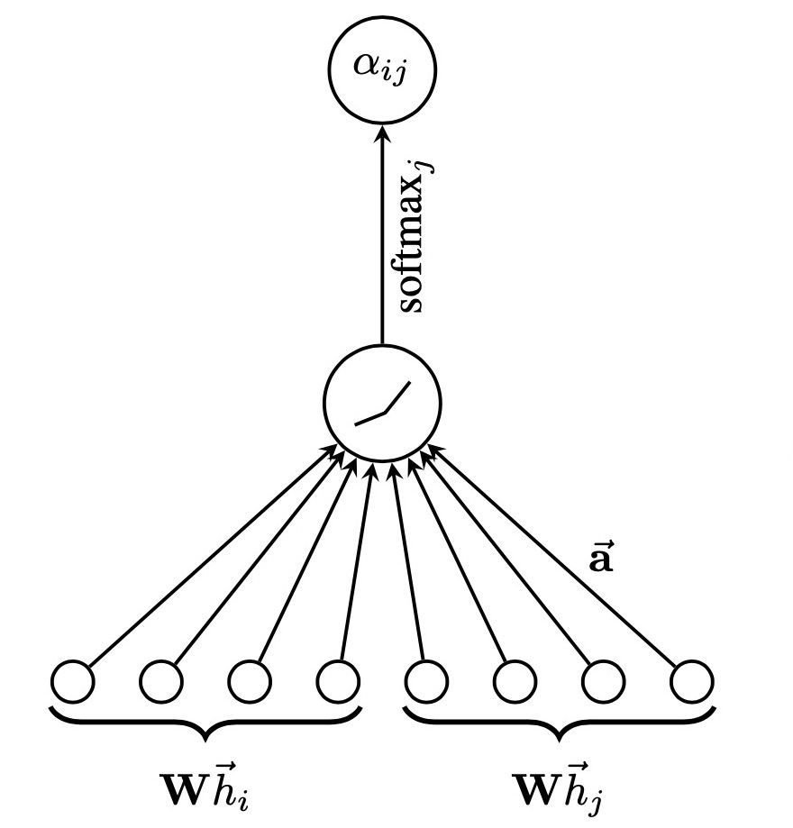
\[\alpha_{ij}=\text{softmax}_j(e_{ij})=\frac{\exp(e_{ij})}{\sum_{k\in\mathcal{N}_i}\exp(e_{ik})}\]实验之中,注意力机制 $a$ 是一个单层的前馈神经网络,通过权值向量来确定模型权重 $\vec{a}\in \reals^{2F’}$,并且加入了 $\text{LeakyRelu}$ 的非线性激活,小于零斜率为 0.2,大于 0 斜率为 0.1。于是需要求的注意力互相关系数的完整表达式如下:
\[\alpha_{ij}=\frac{ \exp( \text{LeakyRelu}(\vec{a}^T[\mathbf{W}\vec{h_i}\parallel\mathbf{W}\vec{h_j}]) ) }{ \sum_{k\in\mathcal{N}_i}\exp( \text{LeakyRelu}(\vec{a}^T[\mathbf{W}\vec{h_i}\parallel\mathbf{W}\vec{h_k}]) ) }\]其中 $^T$ 代表转置,$\parallel$ 表示并列(concatenation)运算。
公式含义就是权值矩阵与 $F’$ 个特征相乘,然后节点相乘后并列在一起,与权重相乘,$\text{LeakyRelu}$ 激活后指数操作得到 $\text{softmax}$ 的分子(分母同理)。
值得一提的是,这篇论文的早期版本里没有使用 $\text{LeakyRelu}$ 进行激活操作。对于对于每条边$(i,j)$,分别将节点 $i$ 和 $j$ 的特征变换为 1 个标量 $f(i)$ 和 $f(j)$ ,然后相加作为未归一化权重。然而后续进行 $\text{softmax}$ 时,传入函数的形式如下:
\[\frac{ \exp(f(i)+f(j)) }{ \sum_{k\in\mathcal{N}_i}\exp(f(i)+f(k)) }\]约去 $\exp(f(i))$ 后得到
\[\frac{ \exp(f(j)) }{ \sum_{k\in\mathcal{N}_i}\exp(f(k)) }\]这表明邻节点的重要性与当前节点无关,只与邻节点自身特征有关。这样忽视了节点本身,就容易导致矩阵在行上相似甚至相等,显然是有问题的。因此,我推测新版论文里加了激活函数可用于破坏上面的公式,使得 $i$ 不能约去。
通过上面,运算得到了正则化后的不同节点之间的注意力互相关系数(normalized attention coefficients),可以用来预测每个节点的输出特征:
\[\vec{h_i'}=\sigma(\sum_{j\in\mathcal{N}_i}\alpha_{ij}\mathbf{W}\vec{h_j})\]这个公式的含义就是节点的输出特征是相邻的所有节点的线性和的非线性激活,线性和的系数是前面求得的注意力互相关系数。
在上面的输出特征加入计算 multi-head 的运算公式:
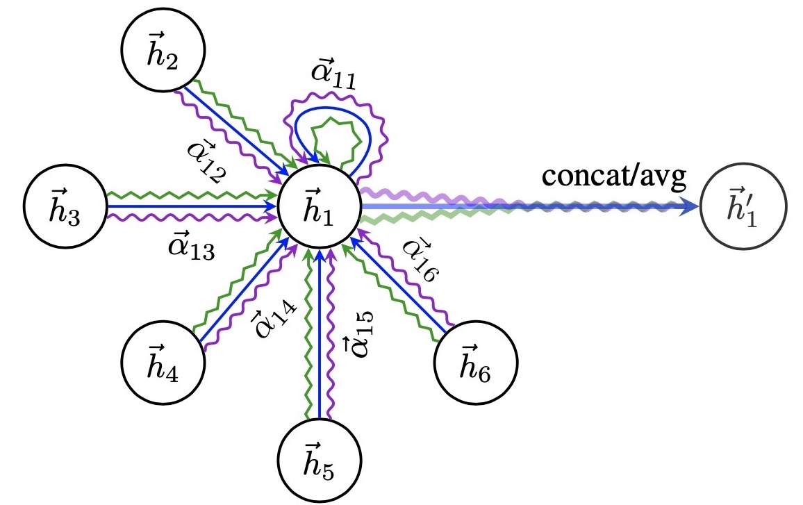
\[\vec{h_i'}=\parallel_{k=1}^K\sigma(\sum_{j\in \mathcal{N}_i}\alpha_{ij}^k\mathbf{W}^k\vec{h_j})\]其中 concate 操作为 $\parallel$ ,$a_{ij}^k$ 是第 $k$ 个注意力机制 $(a_k)$ 算出的正则化注意力互相关系数,$\mathbf{W}^k$ 是对应的权重矩阵,共 $K$ 个注意力机制需要考虑,每个节点输出 $KF’$ 个特征。例如,$K=3$ 时结构如下,节点 1 在邻域中具有多端注意机制,不同的箭头样式表示独立的注意力计算,通过连接或平均每个 head 获取 $\vec{h_1’}$:
对于最终的输出,concate 操作可能不那么敏感了,所以作者直接用 K 平均来取代 concate 操作,得到最终的公式:
\[\vec{h_i'}=\sigma(\frac{1}{K}\sum_{k=1}^K\sum_{j\in\mathcal{N}_i}\alpha_{ij}^k\mathbf{W}^k\vec{h_j})\]实验过程
原论文中的实验分成两部分,半监督学习(transductive learning)和归纳学习(inductive learning)。限于文章篇幅,这里我只放出半监督学习的部分,归纳学习中对于论文中核心的图注意力层的原理是相同的,也可以查看文末参考链接部分原作者的代码。
实验环境
使用的机器没有 cuda 环境,好在即使是在 cpu 上也能很快(1 分钟左右)训练完这个模型。
- Intel(R) Core(TM) i7-6567U CPU @3.30GHZ 3.31GHz
- 8.00GB RAM
- Python 3.8.2 64-bit
- jupyter==1.0.0
- numpy==1.18.4
- torch==1.5.0+cpu
- torch-scatter==2.0.4
- torch-sparse==0.6.4
- torch-cluster==1.5.4
- torch-geometric==1.5.0
导入相关包和数据集
这里我没有选用原作者的代码(见参考部分),而是使用了 PyTorch Geometric 库,其优点是设计了一种新的表示图数据的存储结构,只会为存在的边进行计算,而完全不需要将计算浪费在不存在的边上。相对于原作者直接使用的邻接矩阵(浪费大量的时间为没有边的节点对计算权重,然而在第二步中被 Mask 消去),在我的机器上可以把训练模型的时间缩短到一分钟以内(Cora 数据集)。
1
2
3
4
5
6
7
8
9
10
11
12
13
import torch
from torch import nn
from torch_geometric.data import Data
from torch_geometric.datasets import Planetoid
from torch_geometric import transforms

torch.manual_seed(2020) # seed for reproducible numbers
name_data = 'Cora'
dataset = Planetoid(root= './dataset/' + name_data, name = name_data)
dataset.transform = transforms.NormalizeFeatures()

print(f"Number of Classes in {name_data}:", dataset.num_classes)
print(f"Number of Node Features in {name_data}:", dataset.num_node_features)
注意到下述代码会直接访问 kimiyoung/planetoid 下载所需要的数据集到当前目录下,国内网络环境下有时需要挂上代理,否则会在运行时报「连接断开」的错误。
1
2
Number of Classes in Cora: 7
Number of Node Features in Cora: 1433
图注意力层
torch_geometric包已经实现了所需的图注意力图层,以下内容可以由一句 from torch_geometric.nn import GATConv 简单代替。但是作为对这篇论文本身的学习,还是有必要贴出对应的源码。
1
2
3
4
5
6
7
8
9
10
11
12
13
14
15
16
17
18
19
20
21
22
23
24
25
26
27
28
29
30
31
32
33
34
35
36
37
38
39
40
41
42
43
44
45
46
47
48
49
50
51
52
53
54
55
56
57
58
59
60
61
62
63
64
65
66
67
68
69
70
71
72
73
74
75
76
77
78
79
80
81
82
83
84
85
86
87
88
89
# https://github.com/rusty1s/pytorch_geometric/blob/master/torch_geometric/nn/conv/gat_conv.py
import torch
from torch.nn import Parameter, Linear
from torch_geometric.nn.conv import MessagePassing
from torch_geometric.utils import remove_self_loops, add_self_loops, softmax

from torch_geometric.nn.inits import glorot, zeros

class GATConv(MessagePassing):
    def __init__(self, in_channels, out_channels, heads=1, concat=True,
                 negative_slope=0.2, dropout=0, bias=True, **kwargs):
        super(GATConv, self).__init__(aggr='add', **kwargs)

        self.in_channels = in_channels
        self.out_channels = out_channels
        self.heads = heads
        self.concat = concat
        self.negative_slope = negative_slope
        self.dropout = dropout

        self.__alpha__ = None

        self.lin = Linear(in_channels, heads * out_channels, bias=False)

        self.att_i = Parameter(torch.Tensor(1, heads, out_channels))
        self.att_j = Parameter(torch.Tensor(1, heads, out_channels))

        if bias and concat:
            self.bias = Parameter(torch.Tensor(heads * out_channels))
        elif bias and not concat:
            self.bias = Parameter(torch.Tensor(out_channels))
        else:
            self.register_parameter('bias', None)

        self.reset_parameters()

    def reset_parameters(self):
        glorot(self.lin.weight)
        glorot(self.att_i)
        glorot(self.att_j)
        zeros(self.bias)

    def forward(self, x, edge_index, return_attention_weights=False):
        """"""

        if torch.is_tensor(x):
            x = self.lin(x)
            x = (x, x)
        else:
            x = (self.lin(x[0]), self.lin(x[1]))

        edge_index, _ = remove_self_loops(edge_index)
        edge_index, _ = add_self_loops(edge_index,
                                       num_nodes=x[1].size(self.node_dim))

        out = self.propagate(edge_index, x=x,
                             return_attention_weights=return_attention_weights)

        if self.concat:
            out = out.view(-1, self.heads * self.out_channels)
        else:
            out = out.mean(dim=1)

        if self.bias is not None:
            out = out + self.bias

        if return_attention_weights:
            alpha, self.__alpha__ = self.__alpha__, None
            return out, (edge_index, alpha)
        else:
            return out

    def message(self, x_i, x_j, edge_index_i, size_i,
                return_attention_weights):
        # Compute attention coefficients.
        x_i = x_i.view(-1, self.heads, self.out_channels)
        x_j = x_j.view(-1, self.heads, self.out_channels)

        alpha = (x_i * self.att_i).sum(-1) + (x_j * self.att_j).sum(-1)
        alpha = torch.nn.functional.leaky_relu(alpha, self.negative_slope)
        alpha = softmax(alpha, edge_index_i, size_i)

        if return_attention_weights:
            self.__alpha__ = alpha

        # Sample attention coefficients stochastically.
        alpha = torch.nn.functional.dropout(alpha, p=self.dropout, training=self.training)

        return x_j * alpha.view(-1, self.heads, 1)
我们只需要关注其 forward 过程中会调用的 message 方法:
1
2
3
4
5
6
7
8
alpha = (x_i * self.att_i).sum(-1) + (x_j * self.att_j).sum(-1)
alpha = torch.nn.functional.leaky_relu(alpha, self.negative_slope)
alpha = softmax(alpha, edge_index_i, size_i)

# Sample attention coefficients stochastically.
alpha = torch.nn.functional.dropout(alpha, p=self.dropout, training=self.training)

return x_j * alpha.view(-1, self.heads, 1)
这里算出了前面论文中提到的 $\alpha_{ij}$,然后进行 dropout 操作,相当于计算每个 node 位置的卷积时都是随机的选取了一部分近邻节点参与卷积,可以比较有效的缓解过拟合的发生,在一定程度上达到正则化的效果。最后返回 dropout 后卷积的结果。
模型
- 两层 GATLayer
- 第一层 8 head,$F’=8$,使用 elu(exponential linear unit)作为非线性函数
- 第二层为分类层,一个 attention head,特征数就是类别数,后面跟着 $\text{softmax}$ 函数
- 两层都采用 0.6 的 dropout
1
2
3
4
5
6
7
8
9
10
11
12
13
14
15
16
17
18
19
20
21
22
23
24
25
class GAT(nn.Module):
    def __init__(self):
        super(GAT, self).__init__()
        self.hid = 8
        self.in_head = 8
        self.out_head = 1

        self.conv1 = GATConv(dataset.num_features, self.hid, heads=self.in_head, dropout=0.6)
        self.conv2 = GATConv(self.hid*self.in_head, dataset.num_classes, concat=False,
                             heads=self.out_head, dropout=0.6)


    def forward(self, data):
        x, edge_index = data.x, data.edge_index

        # Dropout before the GAT layer is used to avoid overfitting in small datasets like Cora.
        # One can skip them if the dataset is sufficiently large.

        x = nn.functional.dropout(x, p=0.6, training=self.training)
        x = self.conv1(x, edge_index)
        x = nn.functional.elu(x)
        x = nn.functional.dropout(x, p=0.6, training=self.training)
        x = self.conv2(x, edge_index)

        return nn.functional.log_softmax(x, dim=1)
训练
为了应对数据集小的问题,训练时使用了 weight_decay=5e-4 的 $L_2$ 正则化。
1
2
3
4
5
6
7
8
9
10
11
12
13
14
15
16
17
18
device = torch.device('cuda' if torch.cuda.is_available() else 'cpu')

data = dataset[0].to(device)
model = GAT().to(device)
optimizer = torch.optim.Adam(model.parameters(), lr=0.005, weight_decay=5e-4)

model.train()
for epoch in range(1000):
    model.train()
    optimizer.zero_grad()
    out = model(data)
    loss = nn.functional.nll_loss(out[data.train_mask], data.y[data.train_mask])

    if epoch%200 == 0:
        print(loss)

    loss.backward()
    optimizer.step()
1
2
3
4
5
tensor(1.9447, grad_fn=<NllLossBackward>)
tensor(0.6848, grad_fn=<NllLossBackward>)
tensor(0.6022, grad_fn=<NllLossBackward>)
tensor(0.5589, grad_fn=<NllLossBackward>)
tensor(0.4930, grad_fn=<NllLossBackward>)
评估效果
1
2
3
4
5
model.eval()
_, pred = model(data).max(dim=1)
correct = float(pred[data.test_mask].eq(data.y[data.test_mask]).sum().item())
acc = correct / data.test_mask.sum().item()
print('Accuracy: {:.4f}'.format(acc))
1
Accuracy: 0.8210
总结
GAT 其实就是用注意力机制来计算聚合周边节点时的权重。受益于注意力机制,GAT 能够过滤噪音邻居,改进图卷积的缺点提升模型表现并可以对结果实现一定的解释。此外,GAT 不需要事先知道图结构,也可以应用在动态图上,无疑大大扩展了 GCN 的适用面。
主要参考文献
Related posts