数字图像处理·实验二
post on 26 Sep 2019 about 6485words require 22min
CC BY 4.0 (除特别声明或转载文章外)
如果这些文字帮助到你,可以请我喝一杯咖啡~
PROJECT 04-01 [Multiple Uses] Two-Dimensional Fast Fourier Transform
The purpose of this project is to develop a 2-D FFT program “package” that will be used in several other projects that follow. Your implementation must have the capabilities to:
- Multiply the input image by $(-1)^{x+y}$ to center the transform for filtering.
- Multiply the resulting (complex) array by a real function (in the sense that the the real coefficients multiply both the real and imaginary parts of the transforms). Recall that multiplication of two images is done on pairs of corresponding elements.
- Compute the inverse Fourier transform.
- Multiply the result by $(-1)^{x+y}$ and take the real part.
- Compute the spectrum.
Basically, this project implements Fig. 4.5. If you are using MATLAB, then your Fourier transform program will not be limited to images whose size are integer powers of 2. If you are implementing the program yourself, then the FFT routine you are using may be limited to integer powers of 2. In this case, you may need to zoom or shrink an image to the proper size by using the program you developed in Project 02-04.
An approximation: To simplify this and the following projects (with the exception of Project 04-05), you may ignore image padding (Section 4.6.3). Although your results will not be strictly correct, significant simplifications will be gained not only in image sizes, but also in the need for cropping the final result. The principles will not be affected by this approximation.
原理
- 因为$\Im[f(x,y)(-1)^{x+y}]=F(u-M/2,v-N/2)$,因此频率域的中心平移可以由原图乘上$(-1)^{x+y}$实现。
- 直接在得到的复数数组上乘上实函数即可。
- 可以调用 matlab 的 ifft2
- 同(1),获取实部可以用
real函数 - 复数的模可以用
abs函数
代码
1
2
3
4
5
6
7
8
9
10
11
12
13
14
15
16
17
18
19
20
21
22
23
f=imread('Fig0418(a).tif');%输入图片
H=imread('Fig0418(a).tif');%实函数

[M,N]=size(f);
P=2*M;Q=2*N;

fp=zeros(P,Q);
fp(1:M,1:N)=f(1:M,1:N);%图像填充

[Y,X]=meshgrid(1:Q,1:P);
ones=(-1).^(X+Y);

F=fft2(ones.*fp);%用(-1)^(x+y)乘以输入图像,来实现中心化变换
%(-1)^(x+y)*f(x,y)的傅里叶变换等于fftshift(fft2(f,P,Q));
% 因此上面可用一句F=fftshift(fft2(f,P,Q)); 代替

G=H.*F;%频率域相乘,这里H是实函数

g=real(ifft2(G));%反变换并取结果的实部
g=ones.*g;
g=g(1:M,1:N);%在g(x,y)提取M*N左上象限

I=abs(F);% 取频谱,即模长,直接调用abs即可
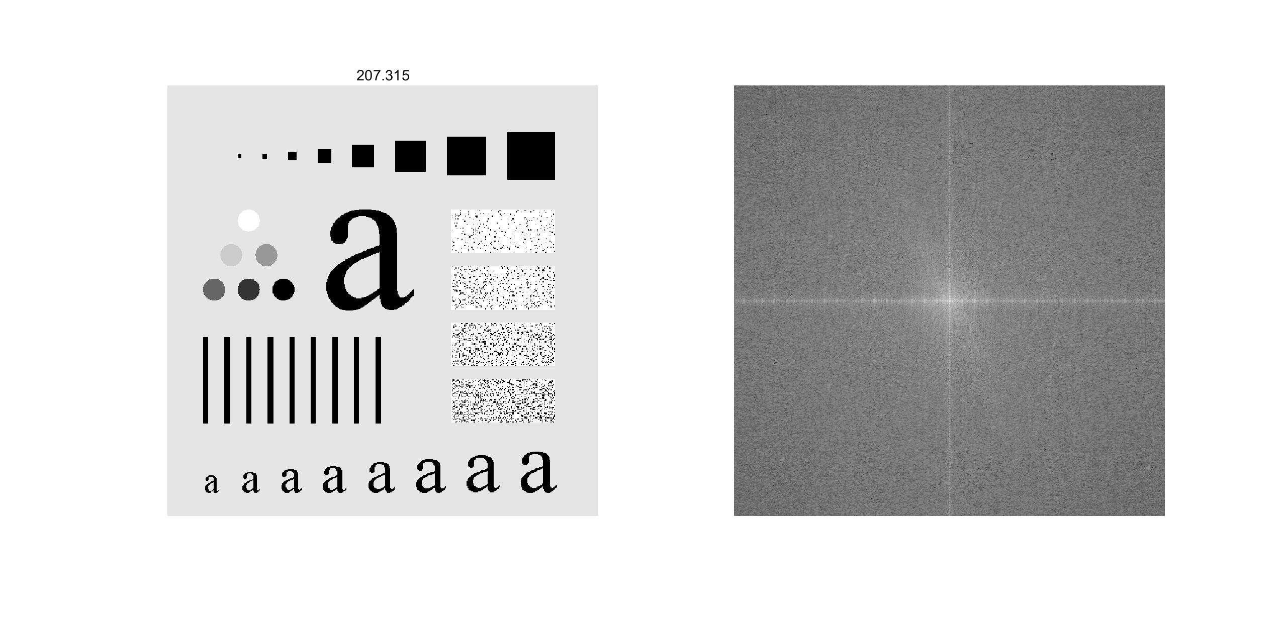
PROJECT 04-02 Fourier Spectrum and Average Value
- Download Fig. 4.18(a) and compute its (centered) Fourier spectrum.
- Display the spectrum.
- Use your result in (a) to compute the average value of the image.
原理
直流分量$F(0,0)=\frac{1}{MN}\sum_{x=0}^M\sum_{y=0}^N$为图像像素的均值。
代码
为了能够更加清楚显示频谱图的情况,输出频谱图的时候做了一次对数变换。
1
2
3
4
5
6
7
8
9
close all;clear all;clc;
I = imread('Fig0418(a).tif');
I = double(I);
[m,n] = size(I);
s = sum(sum(I));
avg = s / (m * n);
subplot(1,2,1),imshow(uint8(I)),title(avg);
sp = abs(fftshift(fft2(I,2*m,2*n)));
subplot(1,2,2),imshow(uint8(log(1 + sp)),[]);
结果
如图,计算出的平均值为 207.315。
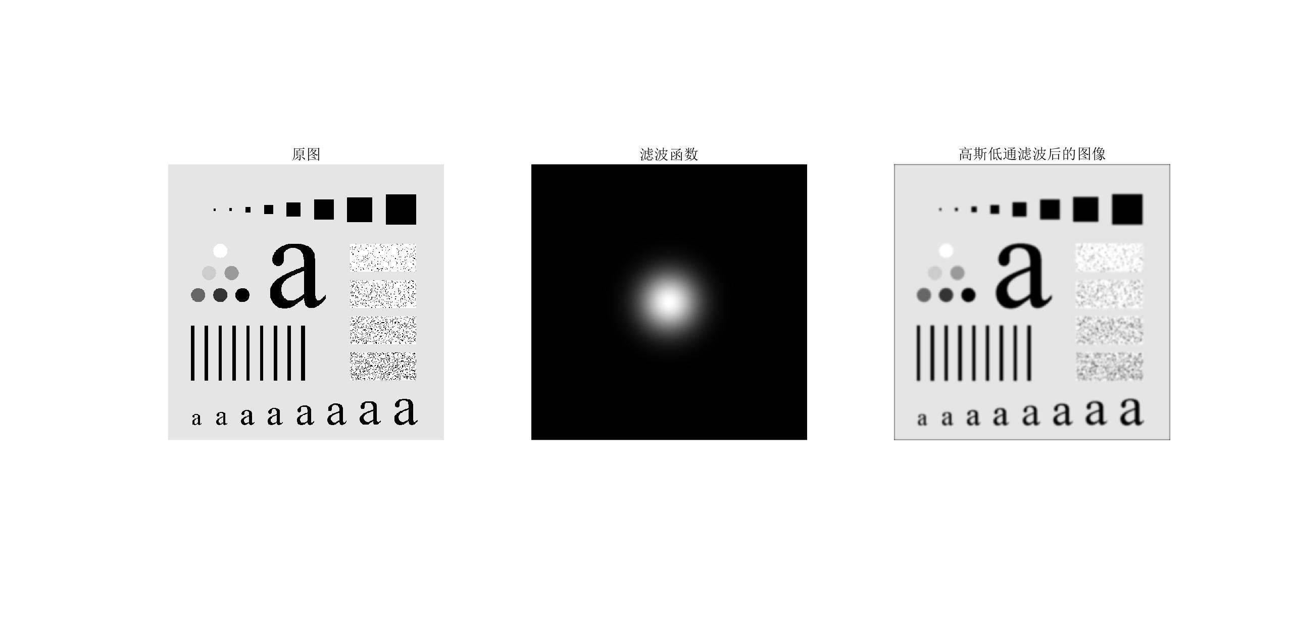
PROJECT 04-03 Lowpass Filtering
- Implement the Gaussian lowpass filter in Eq. (4.3-7). You must be able to specify the size, M x N, of the resulting 2D function. In addition, you must be able to specify where the 2D location of the center of the Gaussian function.
- Download Fig. 4.11(a) [this image is the same as Fig. 4.18(a)] and lowpass filter it to obtain Fig. 4.18(c).
原理
二维高斯滤波器的方程为:$H(u,v)=e^{-D^2(u,v)/2\sigma^2}$,其中$D(u,v)$为距傅里叶变换原点的距离,$\sigma$为高斯曲线扩展的程度。
代码
这里大部分内容可以复用第一问的的代码。
1
2
3
4
5
6
7
8
9
10
11
12
13
14
15
16
17
18
19
20
21
22
23
24
25
26
27
28
29
30
31
32
33
34
35
close all;clear all;clc;
f = imread('Fig0418(a).tif');
f = mat2gray(f);
[M,N] = size(f);
P = 2 * M; Q = 2*N;

%生成实的对称的滤波函数H,中心在(M,N)
alf=100;
for i=1:P
    for j=1:Q
        H(i,j) =exp(-((i-P/2)^2+(j-Q/2)^2)/(2*alf^2));
    end
end


fp=zeros(P,Q);
fp(1:M,1:N)=f(1:M,1:N);%图像填充

[Y,X]=meshgrid(1:Q,1:P);
ones=(-1).^(X+Y);

F=fft2(ones.*fp);%用(-1)^(x+y)乘以输入图像,来实现中心化变换
%(-1)^(x+y)*f(x,y)的傅里叶变换等于fftshift(fft2(f,P,Q));
% 因此上面可用一句F=fftshift(fft2(f,P,Q)); 代替

G=H.*F;%频率域相乘,这里H是实函数

g=real(ifft2(G));%反变换并取结果的实部
g=ones.*g;
g=g(1:M,1:N);%在g(x,y)提取M*N左上象限


subplot(1,3,1),imshow(f),title('原图');
subplot(1,3,2),imshow(H),title('滤波函数');
subplot(1,3,3),imshow(g),title('高斯低通滤波后的图像');
结果
PROJECT 04-04 Highpass Filtering Using a Lowpass Image
- Subtract your image in Project 04-03(b) from the original to obtain a sharpened image, as in Eq. (4.4-14). You will note that the resulting image does not resemble the Gaussian highpass results in Fig. 4.26. Explain why this is so.
- Adjust the variance of your Gaussian lowpass filter until the result obtained by image subtraction looks similar to Fig. 4.26(c). Explain your result.
原理
利用下式可以得到高通滤波的图像
$f_{hp}(x,y)=f(x,y)-f_{lp}(x,y)$
其中$f_{lp}$即为 PROJECT 04-03,即上一个通过高斯滤波后的图像。
代码
在上一问的基础上继续做即可,用原图图像减去高斯低通滤波处理的图像。
1
2
3
4
5
6
7
8
9
10
11
12
13
14
15
16
17
18
19
20
21
22
23
24
25
26
27
28
29
30
31
32
33
34
35
36
37
close all;clear all;clc;
f = imread('Fig0418(a).tif');
f = mat2gray(f);
[M,N] = size(f);
P = 2 * M; Q = 2*N;

%生成实的对称的滤波函数,中心在(M,N)
alf=100;%第二问把这里改成200
for i=1:P
    for j=1:Q
        H(i,j) =exp(-((i-P/2)^2+(j-Q/2)^2)/(2*alf^2));
    end
end

fp=zeros(P,Q);
fp(1:M,1:N)=f(1:M,1:N);%图像填充

[Y,X]=meshgrid(1:Q,1:P);
ones=(-1).^(X+Y);

F=fft2(ones.*fp);%用(-1)^(x+y)乘以输入图像,来实现中心化变换
%(-1)^(x+y)*f(x,y)的傅里叶变换等于fftshift(fft2(f,P,Q));
% 因此上面可用一句F=fftshift(fft2(f,P,Q)); 代替

G=H.*F;%频率域相乘,这里H是实函数

g=real(ifft2(G));%反变换并取结果的实部
g=ones.*g;
g=g(1:M,1:N);%在g(x,y)提取M*N左上象限


subplot(2,2,1),imshow(f),title('原图');
subplot(2,2,2),imshow(H),title('滤波函数');
subplot(2,2,3),imshow(g),title('高斯低通滤波后的图像');

g=im2double(g);f=im2double(f);gmask=f-g;
subplot(2,2,4),imshow(gmask);title('钝化模板');
结果
用原图减去高斯低通滤波处理后的图像后确实变模糊了。和课本上的图片对比,我这里生成的图片边缘更加清楚一些(主观上感觉)。如果排除印刷的问题,考虑到公式上与直接做高斯高通滤波是等价的,可能是因为不同的计算方式导致了不同的浮点数误差造成的。
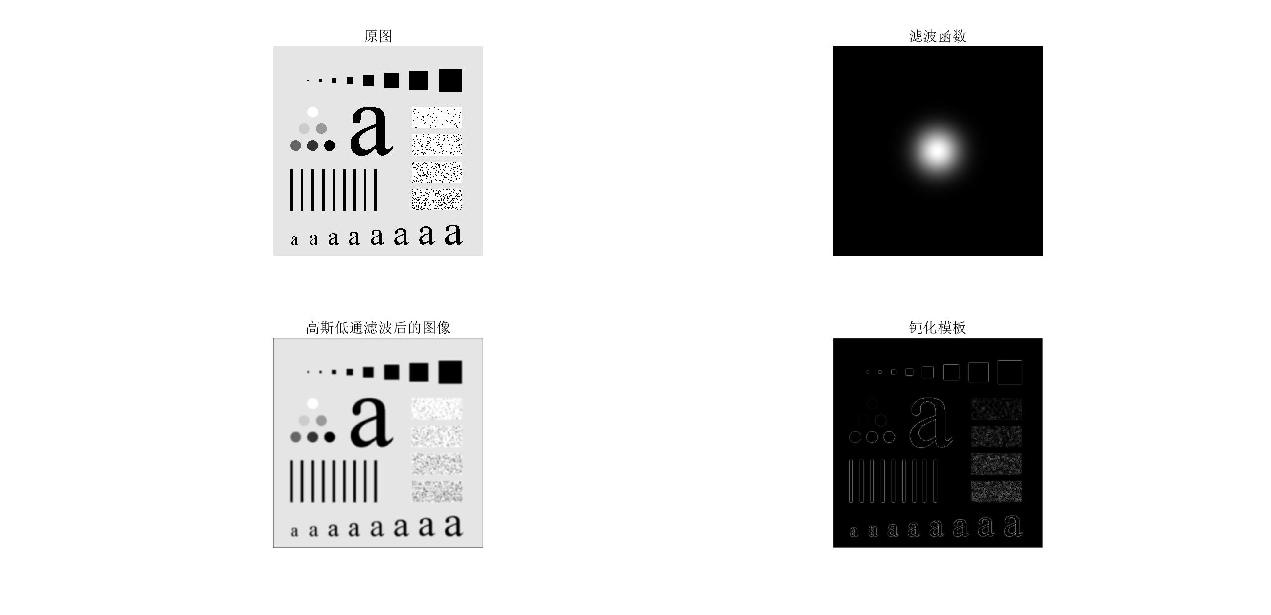
调整第 8 行为alf=200,可以看到模板变得更模糊了,更加接近课本。
PROJECT 04-05 Correlation in the Frequency Domain
Download Figs. 4.41(a) and (b) and duplicate Example 4.11 to obtain Fig. 4.41(e). Give the (x,y) coordinates of the location of the maximum value in the 2D correlation function. There is no need to plot the profile in Fig. 4.41(f).
代码
1
2
3
4
5
6
7
8
9
10
11
12
13
14
15
16
17
18
19
20
21
22
23
24
close all;clc;clear all;
f1 = imread('Fig4.41(a).jpg');
f2 = imread('Fig4.41(b).jpg');
[M1, N1] = size(f1);
[M2, N2] = size(f2);
P = 298;
Q = 298;
[Y,X]=meshgrid(1:Q,1:P);
ones=(-1).^(X+Y);
fp1 = zeros(P, Q);
fp2 = zeros(P, Q);
fp1(1:M1, 1:N1) = f1(1:M1, 1:N1);
fp2(1:M2, 1:N2) = f2(1:M2, 1:N2);
Fp1 = fft2(ones.*fp1);
Fp2 = fft2(ones.*fp2);
Fp = Fp2 .* conj(Fp1);% 求共轭
fp = ifft2(Fp);
fp = real( ones.* fp);
fp = mat2gray(fp);
max_value = max(max(fp));
[row,col] = find(fp == max_value);
subplot(1,3,1),imshow(f1),title(['max value is : ', num2str(max_value)]);
subplot(1,3,2),imshow(f2),title(['(', num2str(row), ',', num2str(col),')']);
subplot(1,3,3),imshow(fp);
结果
如图,从左到右分别为原图、掩膜/需要查找的图像、共轭生成的相关图(其实并没有要求输出)。
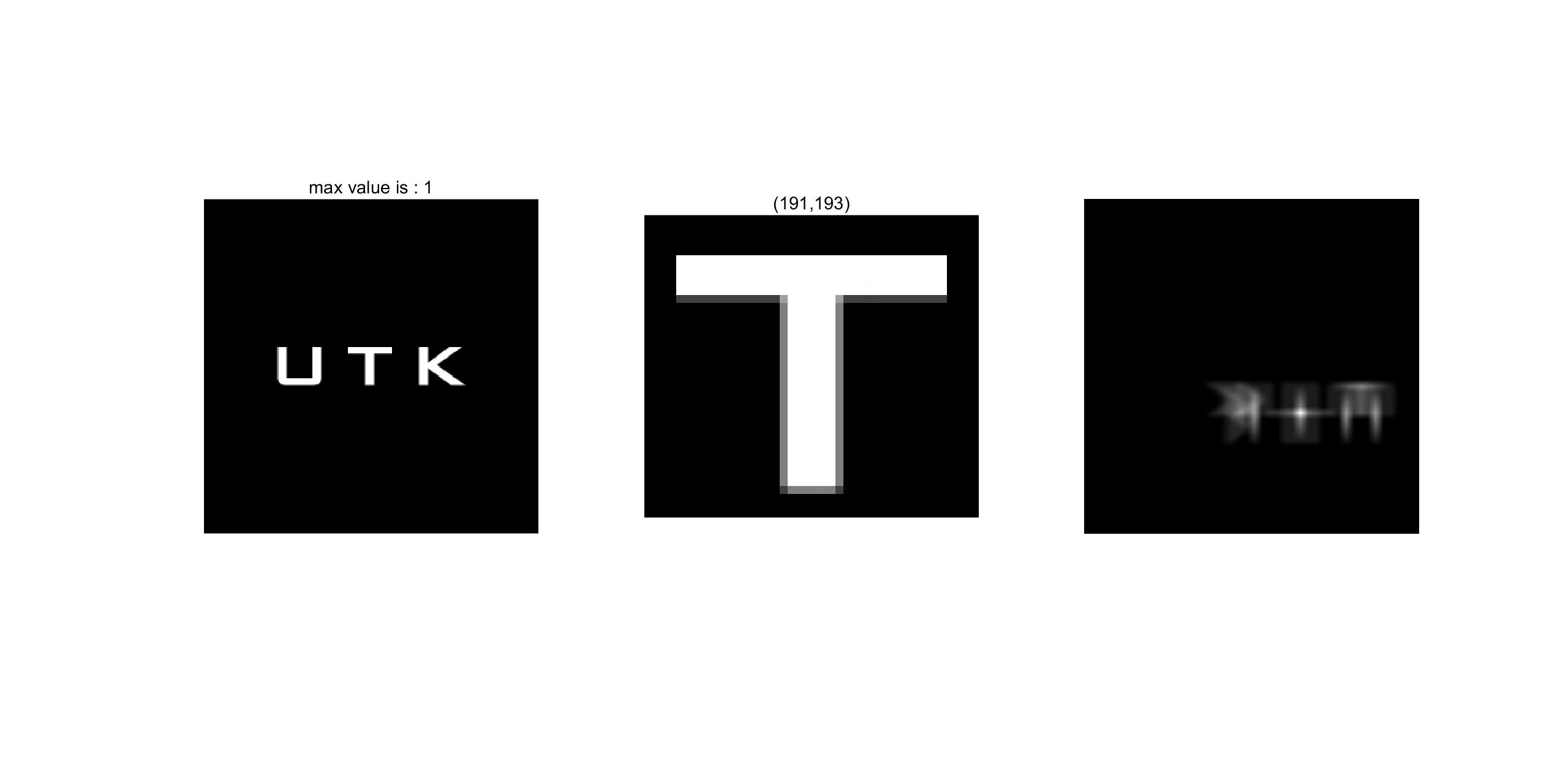
最大值出现在(191,193)的位置,符合预期。
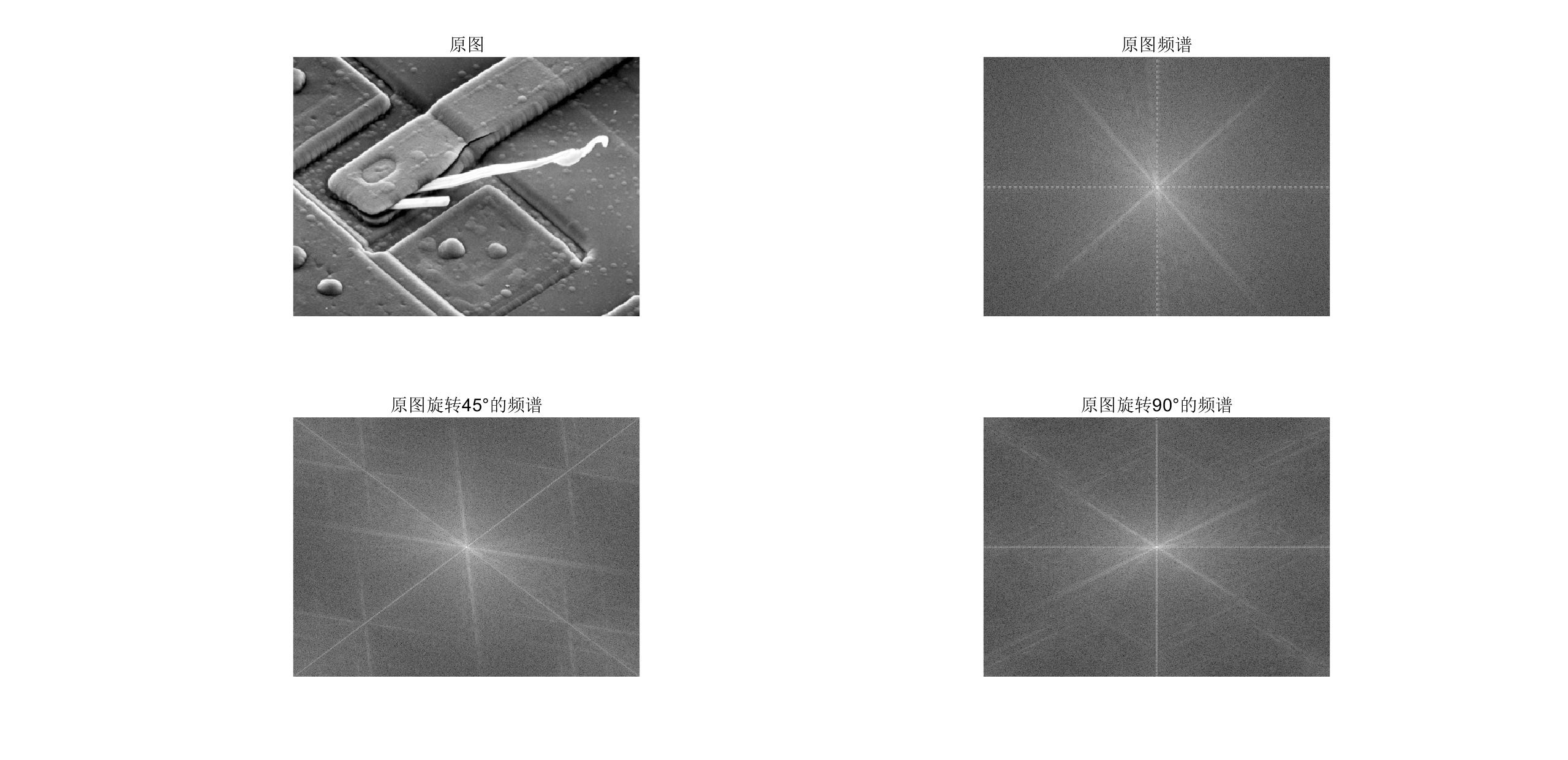
以 figure4.4 为例检验谱平面随着图像旋转而旋转的性质
原理
引入极坐标$x=r\cos\theta,y=r\sin\theta,u=\omega\cos\phi,v=\omega\sin\phi$,计算可得$f(r,\theta+\theta_0)\iff F(\omega,\phi+\theta_0)$
代码
在 PROJECT 04-02 的代码上略作修改即可。
1
2
3
4
5
6
7
8
9
10
11
12
13
14
15
close all;clear all;clc;
I = imread('Fig4.04(a).jpg');
I = double(I);
[m,n] = size(I);
s = sum(sum(I));
avg = s / (m * n);
subplot(2,2,1),imshow(uint8(I)),title('原图');
sp = abs(fftshift(fft2(I,2*m,2*n)));
subplot(2,2,2),imshow(uint8(log(1 + sp)),[]),title('原图频谱');
I=imrotate(I,45);
sp = abs(fftshift(fft2(I,2*m,2*n)));
subplot(2,2,3),imshow(uint8(log(1 + sp)),[]),title('原图旋转45°的频谱');
I=imrotate(I,45);
sp = abs(fftshift(fft2(I,2*m,2*n)));
subplot(2,2,4),imshow(uint8(log(1 + sp)),[]),title('原图旋转90°的频谱');
结果
可以看出,当原图进行旋转时,频谱图确实以相同的角度和方向旋转。
Related posts