数字图像处理·实验一
post on 03 Sep 2019 about 3755words require 13min
CC BY 4.0 (除特别声明或转载文章外)
如果这些文字帮助到你,可以请我喝一杯咖啡~
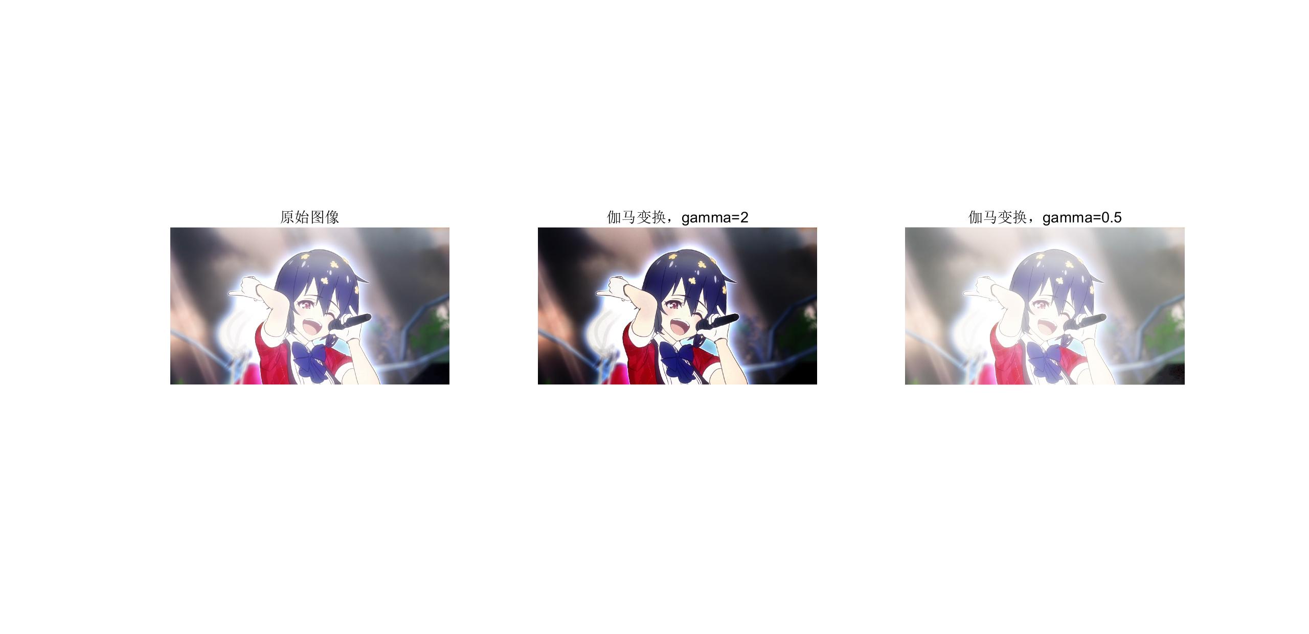
伽马变换
1
2
3
4
5
6
7
8
9
10
11
12
	close all;clc;clear all;
	I=imread('MizunoAi.jpg');
	subplot(1,3,1);imshow(I);title('原始图像');
	c=cat(3,gamma(I(:,:,1),2),gamma(I(:,:,2),2),gamma(I(:,:,3),2));
	subplot(1,3,2);imshow(c);title('伽马变换,gamma=2');
	c=cat(3,gamma(I(:,:,1),0.5),gamma(I(:,:,2),0.5),gamma(I(:,:,3),0.5));
	subplot(1,3,3);imshow(c);title('伽马变换,gamma=0.5');
function J=gamma(I,g)
	c = 255^(1-g);
	J = c * double(I).^g;
	J = mat2gray(J);
end
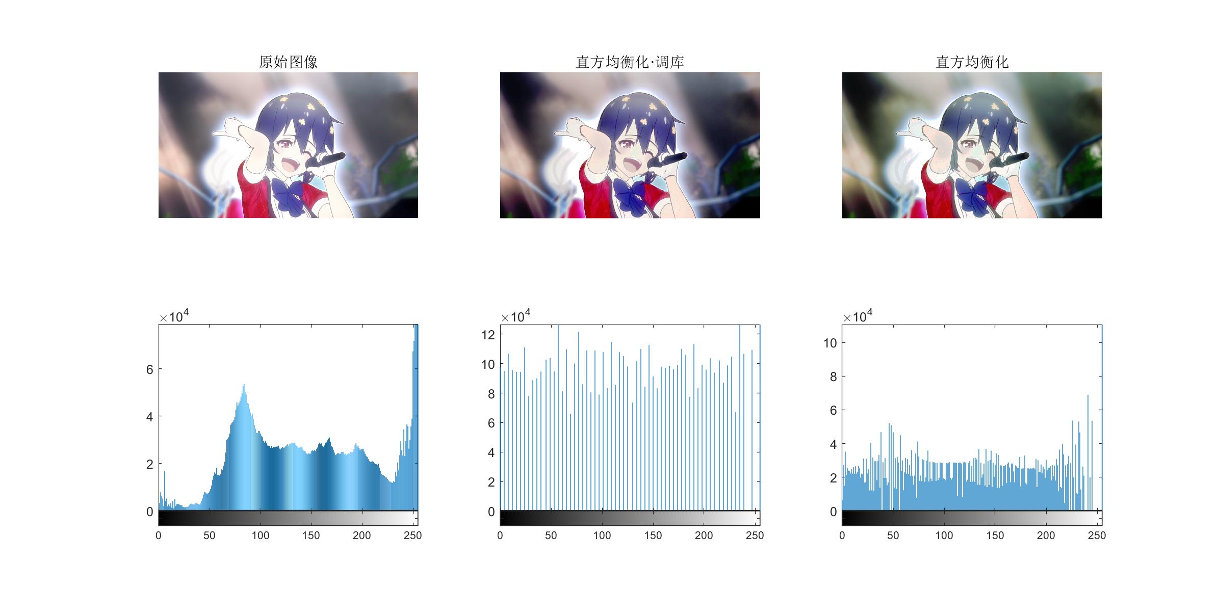
PROJECT 03-02 [Multiple Uses] Histogram Equalization
- Write a computer program for computing the histogram of an image.
- Implement the histogram equalization technique discussed in Section 3.3.1.
- Download Fig. 3.8(a) and perform histogram equalization on it.
As a minimum, your report should include the original image, a plot of its histogram, a plot of the histogram-equalization transformation function, the enhanced image, and a plot of its histogram. Use this information to explain why the resulting image was enhanced as it was.
变换函数是:$s_k=T(r_k)=(L-1)\sum_{j=0}^kp_r(r_j)=(L-1)\sum_{j=0}^k\frac{n_j}{n}$,其中$k=0,1,\dots,L-1$
我想做一些加强,针对彩色图片做直方图均衡化。查了一些网上资料,就是对三维 RGB 图像的三种颜色分别做一次灰度均衡。
1
2
3
4
5
6
7
8
9
10
11
12
13
14
15
16
17
18
19
20
21
22
23
24
25
26
27
28
	I=imread('MizunoAi.jpg');
	subplot(2,3,1);imshow(I);title('原始图像');subplot(2,3,4);imhist(I);
	c=histeq(I);
	subplot(2,3,2);imshow(c);title('直方均衡化·调库');subplot(2,3,5);imhist(c);
	c=cat(3,histogram(I(:,:,1)),histogram(I(:,:,2)),histogram(I(:,:,3)));
	subplot(2,3,3);imshow(c);title('直方均衡化');subplot(2,3,6);imhist(c);
function J=histogram(I)
	J=I;
	[n,m]=size(I);
	a=zeros(1,256);
	b=zeros(1,256);
	for i=1:n
		for j=1:m
			a(1,I(i,j)+1)=a(1,I(i,j)+1)+1;
		end
	end
	sum=0;
	for i=1:256
		sum=sum+a(1,i);
		b(1,i)=255*sum/(m*n);
	end
	for i=1:n
		for j=1:m
			d=J(i,j)+1;
			J(i,j)=b(1,d);
		end
	end
end
运行结果如下,同时输出调用 matlab 自己的直方图均衡函数的结果作为对比,发现自己写的图像均衡偏绿,不知道彩色图像做均衡化要做什么黑科技…不过右侧阴影处的细节确实变得清晰了。
PROJECT 03-05 Enhancement Using the Laplacian
- Use the programs developed in Projects 03-03 and 03-04 to implement the Laplacian enhancement technique described in connection with Eq. (3.7-5). Use the mask shown in Fig. 3.39(d).
- Duplicate the results in Fig. 3.40. You will need to download Fig. 3.40(a).
原理
对连续函数情形,最简单且各向同性的二阶微分算子是拉普拉斯(Laplacian)算子$\triangledown^2f=\frac{\partial^2f}{\partial x^2}+\frac{\partial^2f}{\partial y^2}$。
离散情况下,$\frac{\partial^2f}{\partial x^2}=f(x-1,y)+f(x+1,y)-2f(x,y)$,$\frac{\partial^2f}{\partial y^2}=f(x,y-1)+f(x,y+1)-2f(x,y)$,于是$\triangledown^2f=f(x+1,y)+f(x-1,y)+f(x,y+1)+f(x,y-1)-4f(x,y)$
- 当拉普拉斯算子中心系数为正的时候,有$g(x,y)=f(x,y)+\triangledown^2f$
- 当拉普拉斯算子中心系数为正的时候,有$g(x,y)=f(x,y)-\triangledown^2f$
源代码
1
2
3
4
5
6
7
8
9
10
11
12
13
14
15
16
17
18
close all;clc;
I=imread('liftingbody.png');
I=im2double(I);
J=zeros(size(I));
[M,N]=size(I);
for x=2:M-1
	for y=2:N-1
		J(x,y)=9*I(x,y);
		for dx=-1:1
			for dy=-1:1
				J(x,y)=J(x,y)-I(x+dx,y+dy);
			end
		end
	end
end
subplot(1,3,1);imshow(im2uint8(I));
subplot(1,3,2);imshow(im2uint8(J));
subplot(1,3,3);imshow(im2uint8(I+J));
运行结果
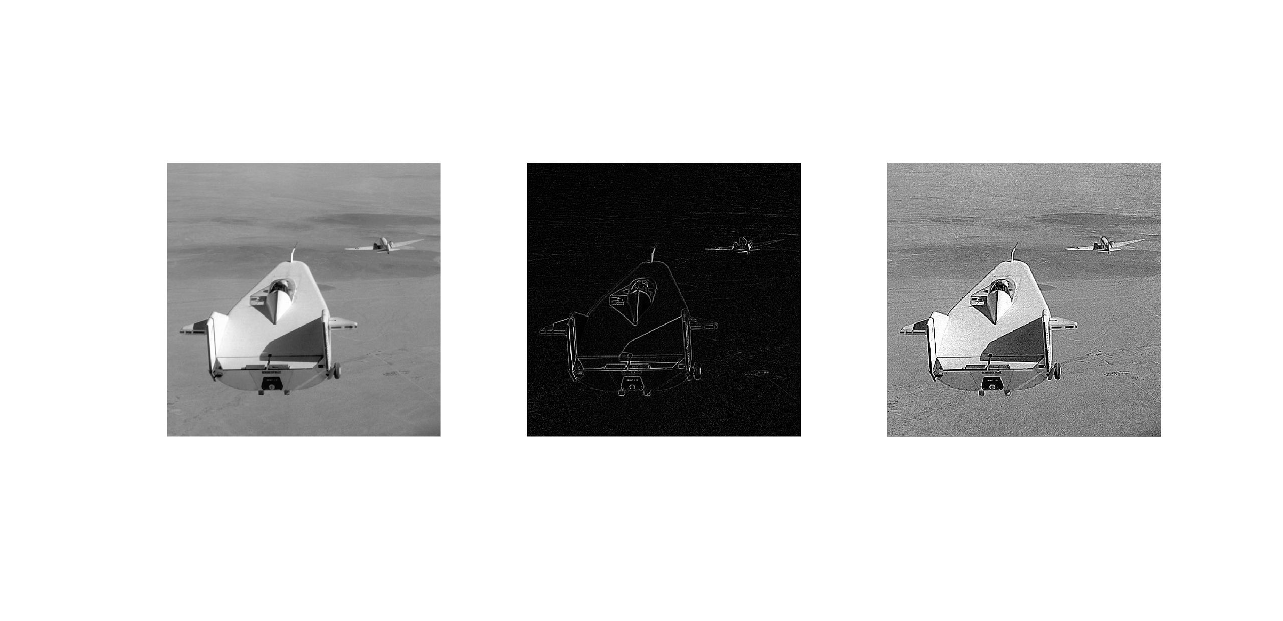
左一是原图,左二是模板,左三是拉普拉斯变换得到的最终图像,可以看到,增强后的第三张图中阴影边缘对比变强了。
PROJECT 03-06 Unsharp Masking
- Use the programs developed in Projects 03-03 and 03-04 to implement highboost filtering, as given in Eq. (3.7-8). The averaging part of the process should be done using the mask in Fig. 3.34(a).
- Download Fig. 3.43(a) and enhance it using the program you developed in (a). Your objective is to choose constant A so that your result visually approximates Fig. 3.43(d).
原理
- 当拉普拉斯算子中心系数为正的时候,有$f_{hb}(x,y)=Af(x,y)+\triangledown^2f$
- 当拉普拉斯算子中心系数为正的时候,有$f_{hb}(x,y)=Af(x,y)-\triangledown^2f$
可以看出,基于拉普拉斯算子的高提升滤波,当$A=1$时就是拉普拉斯图像增强方法,当$A$足够大时,锐化效果将变得不明显
源代码
因为拉普拉斯变换就是特定条件的基于拉普拉斯算子的高提升滤波,所以和上一个代码几乎相同。
1
2
3
4
5
6
7
8
9
10
11
12
13
14
15
16
17
18
close all;clc;
I=imread('liftingbody.png');
I=im2double(I);
J=zeros(size(I));
[M,N]=size(I);
for x=2:M-1
	for y=2:N-1
		J(x,y)=9*I(x,y);
		for dx=-1:1
			for dy=-1:1
				J(x,y)=J(x,y)-I(x+dx,y+dy);
			end
		end
	end
end
subplot(1,3,1);imshow(im2uint8(I+J));
subplot(1,3,2);imshow(im2uint8(1.5*I+J));
subplot(1,3,3);imshow(im2uint8(2*I+J));
运行结果
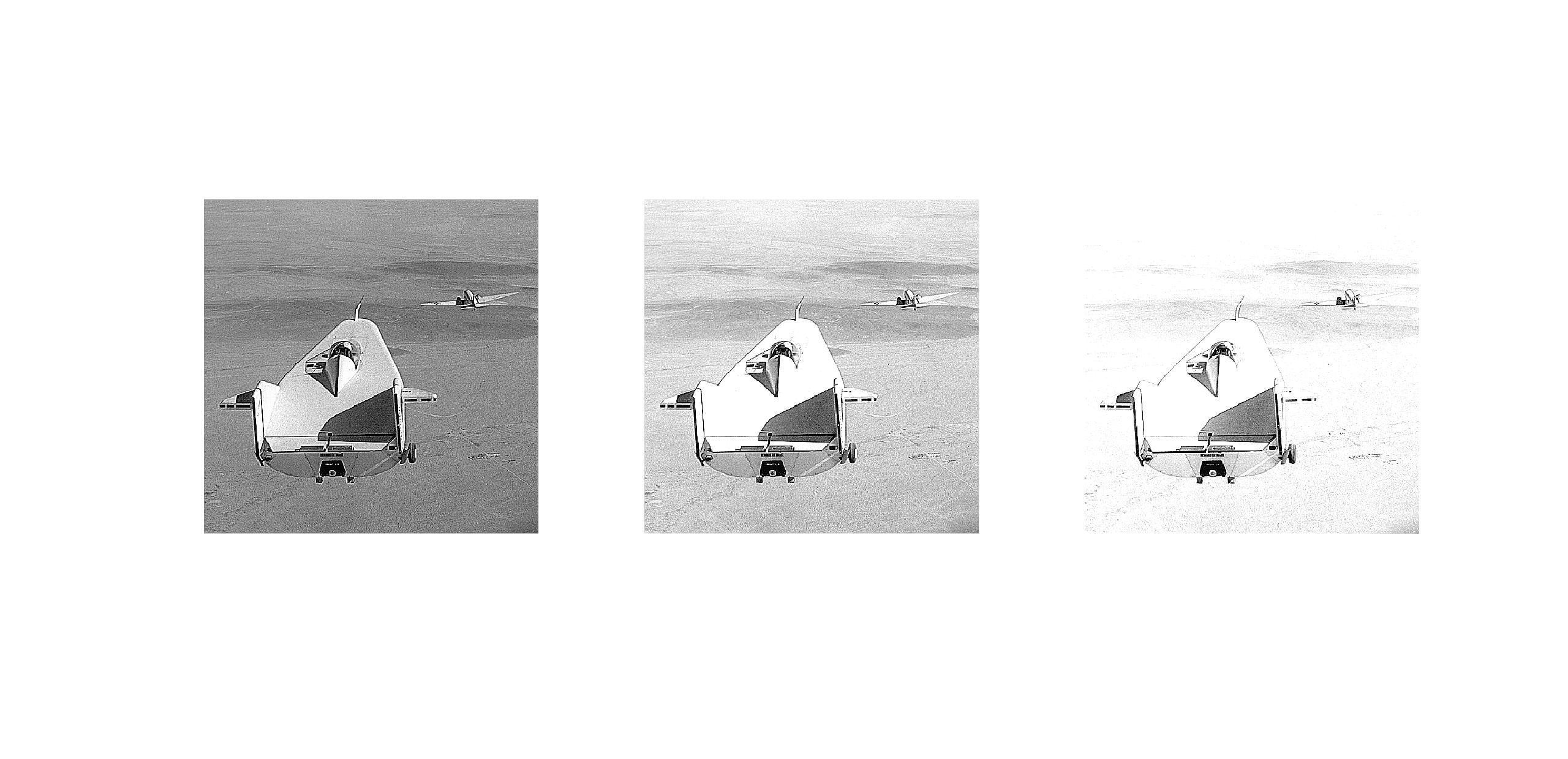
如图,上面三张图自左向右是分别赋值A=1、A=1.5、A=2时的非锐化掩模,其中A=1时就是标准拉普拉斯锐化。自左向右图像的边缘突出效果不断增加。
Related posts