并行与分布式计算·复习笔记
post on 08 Jul 2019 about 80786words require 270min
CC BY 4.0 (除特别声明或转载文章外)
如果这些文字帮助到你,可以请我喝一杯咖啡~
本文档为合作笔记,各讲内容分别由下述成员完成:
由于个人笔记风格不同,水平亦有差异,难免有缺漏、错误的情况出现,如果有疑问、指正欢迎在评论区提出。
第一讲:并行计算概览,内容要点
并行计算主要研究下面几个方面的内容
- 并行架构
- 并行算法
- 并行编程
- 并行性能
- 并行应用
相关基本概念
并行计算可以简单定义为同时利用多个计算资源解决一个计算问题
- 程序运行在多个 CPU 上;
- 一个问题被分解成离散可并发解决的小部分;
- 每一小部分被进一步分解成一组指令序列;
- 每一部分的指令在不同的 CPU 上同时执行;
- 需要一个全局的控制和协调机制;
可并行的计算问题
- 可分解成同时计算的几个离散片段;
- 在任意时刻可同时执行多条指令;
- 多计算资源所花的时间少于单计算资源;
计算资源
一般为:
- 具有多处理器/多核的单台主机;
- 通过网络连接的若干数量的主机
并行计算的优势
- 在自然界,很多复杂的、交叉发生的事件是同时发生的,但是又在同一个时间序列中;
- 与串行计算相比,并行计算更擅长建模、模拟、理解真实复杂的现象
- 节省时间和花费
- 理论上,给一个任务投入更多的资源将缩短任务的完成时间,减少潜在的代价;
- 并行计算机可以由多个便宜、通用计算资源构成;
- 解决更大/更复杂问题:很多问题很复杂,不实际也不可能在单台计算机上解决,例如:Grand Challenges
- 实现并发处理:单台计算机只能做一件事情,而多台计算机却可以同时做几件事情(例如协作网络,来自世界各地的人可以同时工作)
- 利用非本地资源:当本地计算资源稀缺或者不充足时,可以利用甚至是来自互联网的计算资源。
- SETI@home (setiathome.berkeley.edu);
- Folding@home (folding.stanford.edu)
- 更好地发挥底层并行硬件
- 现代计算机甚至笔记本都具有多个处理器或者核心;
- 并行软件就是为了针对并行硬件架构出现的;
- 串行程序运行在现代计算机上会浪费计算资源;
并行计算发展的驱动力
应用发展趋势
在硬件可达到的性能与应用对性能的需求之间存在正反馈(Positive Feedback Cycle)
大数据时代
架构发展趋势
发展过程
迄今为止,CPU 架构技术经历了四代即:电子管(Tube)、晶体管(Transistor)、集成电路(IC)和大规模集成电路(VLSI),这里只关注 VLSI。
VLSI 最的特色是在于对并行化的利用,不同的 VLSI 时代具有不同的并行粒度:
- bit 级并行
- 指令集并行
- 线程水平的并行
其中,有摩尔定律支持芯片行业的发展:「芯片上的集成晶体管数量每 18 个月增加一倍」。
发展趋势的变化
发展趋势不再是高速的 CPU 主频,而是「多核」。(摩尔定律失效的原因之一)
如何提高 CPU 的处理速度
1990 年之前的解决方式
- 增加时钟频率(扩频)
- 深化流水线(采用更多/更短的流水阶段)
- 芯片的工作温度会过高
- 推测超标量(Speculative Superscalar, SS)
多条指令同时执行(指令级的并行,ILP):
- 硬件自动找出串行程序中的能够同时执行的独立指令集合;
- 硬件预测分支指令;在分支指令实际发生之前先推测执行;
局限:最终出现「收益下降(diminishing returns)」 这种解决方法的优点:程序员并不需要知道这些过程的细节
2000 年之后的解决方式
- 时钟频率很难增加;
- SS 触到天花板出现「收益下降」;
- 利用额外的额外的晶体管在芯片上构建更多/更简单的处理器;
后来发展,延申出了并行计算机和并行计算集群。
并行计算机
从硬件角度来讲,今天的单个计算机都是并行计算机,主要体现为:
- 多个功能单元(L1 Cache、L2 Cache、Branch、Prefetch、GPU 等);
- 多个执行单元或者核心
- 多个硬件线程
并行计算集群
多个单独的计算机通过网络连接起来形成计算集群
LLNL 并行计算集群
- 每个节点都是一个多处理器并行机;
- 多个计算节点通过 Infiniband 网络连接;
Moore’s law 新解
- 每两年芯片上的核心数目会翻倍;
- 时钟频率不再增加,甚至是降低;
- 需要处理具有很多并发线程的系统;
- 需要处理芯片内并行和芯片之间的并行;
- 需要处理异构和各种规范(不是所有的核都相同);
最后得出结论,需要程序员学会并行编程。
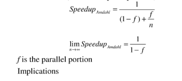
Amdahl’s Law
用于度量并行程序的加速效果
\[Speedup = \frac{1thread\, execution \, time }{n\, thread \, execution \, time}\\ Speedup = \frac{1}{(1-p)+p/n}\\\]其中,p 表示程序可并发的部分占整个程序的比例。
第二讲:并行架构
并行架构
Flynn’s Taxonomy(分类法)
定义:一种并行架构的分类方法
A classification of computer architectures based on the number of streams of instructions and data

SISD Architecture
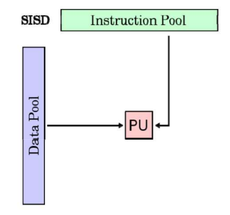
例如:单核计算机
SIMD Architecture:单指令多数据流
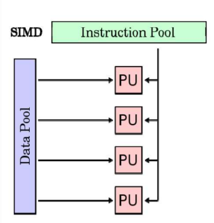
例子:vector processor,GPUs
延申:SPMD,对称多处理器
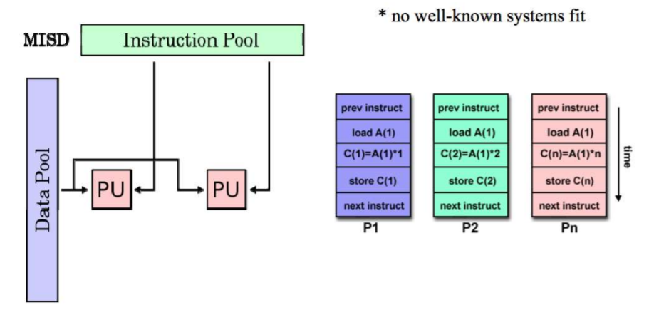
MISD Architecture
多指令单数据流
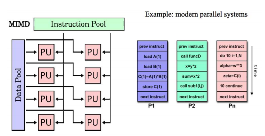
MIMD Architecture 多指令多数据流
单处理器并行(Uniprocessor Parallelism)
引入
How do uniprocessor computer architectures extract parallelism?
- By finding parallelism within instruction stream
- Called 「Instruction Level Parallelism」 (ILP) 指令级并行
- The theory: hide parallelism from programmer
早期的目标
Goal of Computer Architects until about 2002:
- Hide Underlying Parallelism from everyone: OS, Compiler,Programmer
Examples of ILP techniques 指令级并行的技术
- (流水线)Pipelining: Overlapping individual parts of instructions
- (超标量执行)Superscalar execution: Do multiple things at same time
- VLIW: Let compiler specify which operations can run in parallel
- (向量处理)Vector Processing: Specify groups of similar (independent) operations
- (乱序执行) Out of Order Execution (OOO): Allow long operations to happen
流水线技术
Limits to Pipelining
- Overhead prevents arbitrary division (最小可划分部分的时间)
- Cost of latches (between stages) limits what can do within stage
- Sets minimum amount of work/stage
- Hazards prevent next instruction from executing during its designated clock cycle(冒险)
- 结构冒险 Structural hazards: Attempt to use the same hardware to do two different things at once
- 数据冒险 Data hazards: Instruction depends on result of prior instruction still in the pipeline
- 控制冒险 Control hazards: Caused by delay between the fetching of instructions and decisions about changes in control flow (branches and jumps)
乱序执行 Out-of-Order (OOO) Execution
预测执行
最后得知结论,并行需要暴露给程序员,让软件来实现。
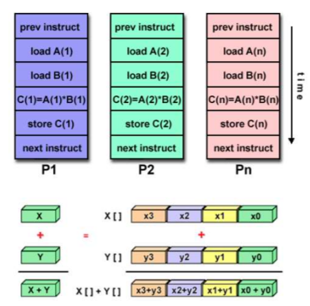
向量处理:VECTOR PROCESSING/SIMD
1. 向量编程模型图解

2. SIMD 架构示意图
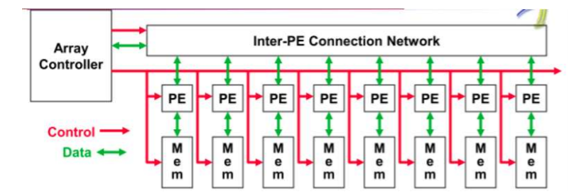
- 中央控制器广播指令给处理单元:Central controller broadcasts instructions to multiple processing elements (PEs)
- 只需一个中央控制器 Only requires one controller for whole array
- 只需要内存存程序的一份代码 Only requires storage for one copy of program
- 计算异步 All computations are fully synchronized
多线程技术 MULTITHREADING:INCLUDING PTHREADS
相关概念
Thread Level Parallelism (TLP) :线程级并行
Concurrency vs Parallelism:并发和并行
介绍 POSIX Threads
定义POSIX: Portable Operating System Interface for UNIX
特点:共享堆,不共享栈
**线程调度:Thread Scheduling **
调度实现方式:
-
多道程序设计 Multitasking operating system
- 硬件多线程
- 切换线程的时机
ILP 与 TLP 关系是什么意思?没看懂
超线程「Simultaneous Multithreading」
定义:既有多线程,又有指令级的并行
超线程,可以更好的占用处理器资源
内存系统 UNIPROCESSOR MEMORY SYSTEMS
内存的限制
- Memory system, and not processor speed, is often the bottleneck for many applications.
- Memory system performance is largely captured by two parameters, latency **and **bandwidth.
- Latency is the time from the issue of a memory request to the time the data is available at the processor.
- Bandwidth is the rate at which data can be pumped to the processor by the memory system
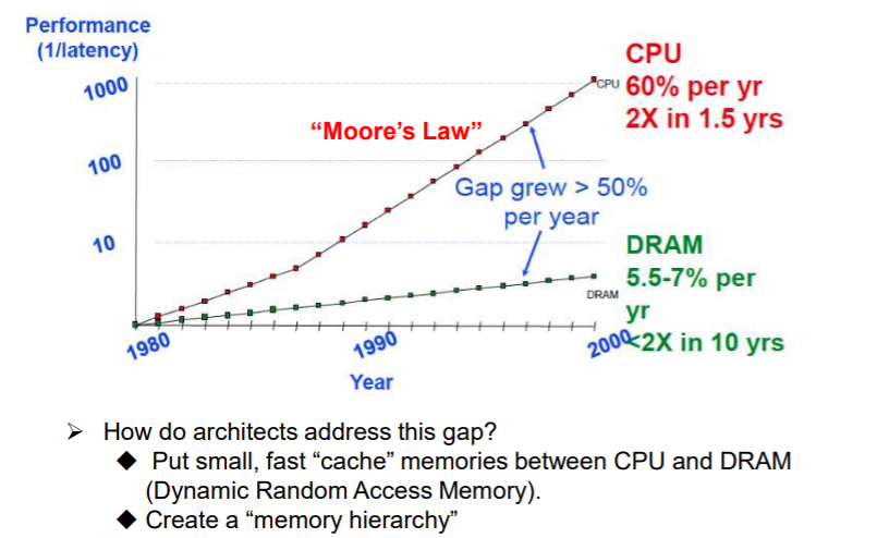
内存墙的问题
局部性原理 Principle of Locality
定义:
Program access a relatively small portion of the address space at any instant of time
-
时间局部性
-
空间局部性
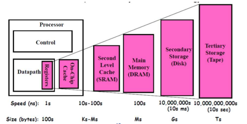
分级存储 Memory Hierarchy
命中率,内存延迟
多核、多处理器 MULTICORE CHIPS
并行架构?WHAT IS PARALLEL ARCHITECTURE
- Machines with multiple processors
-
A parallel computer is a collection of processing elements that cooperate to solve large problems fast Some broad issues
- Resource Allocation
- Data access, Communication and Synchronization
- Performance and Scalability(性能和可伸缩性)
并行领域:A PARALLEL ZOO OF ARCHITECTURES
MIMD Machines
-
定义:Multiple Instruction, Multiple Data (MIMD)
-
通信方式:
-
Shared memory: Communication through Memory
-
Message passing: Communication through Messages
-
For most machines, shared memory built on top of message passing network
举例
Symmetric Multiprocessor
- Multiple processors in box with shared memory communication
- Current MultiCore chips like this
- Every processor runs copy of OS
1. Flynn’s 并行架构分类
- 基于指令流和数据流数量的计算机体系结构分类
SISD 架构:单核计算机 SIMD 架构:向量处理器,GPUs MISD 架构:(没有符合的知名系统。。) MIMD 架构:现代并行系统
2. 什么是 pipeline
- Pipelining
- 流水线有助于带宽而不是延迟
- 带宽受限于最慢的流水线阶段
- 加速潜力 = 流水线级数
- MIPS 流水线的 5 个阶段:Fetch->Decode->Execute->Memory->Write Back
- 流水线 CPI < 1
- 流水线的限制
开销防止任意划分
- 阶段之间锁存器的成本限制了阶段内能做什么
- 设置最小数量的阶段
冒险阻止下一条指令在其指定的时钟周期内执行
- 结构冒险:尝试同时使用相同的硬件执行两个不同的操作
- 数据冒险:指令取决于仍在流水线中先前指令的结果
- 控制冒险:由于控制流程(分支和跳跃)中的指令和决策获取之间的延迟而造成的
超标量增加的冒险的发生
更多冲突的指令(时钟周期)
3. 有哪些形式的指令级并行
- 单处理器计算机体系结构如何提取并行性?
通过在指令流中查找并行性,称为「指令级并行」,向程序员隐藏并行性。
- 指令级并行的例子
- 流水线:指令的各个部分重叠
- 超标量执行:同时执行多个操作
- VLIW(极长指令字):让编译器指定哪些操作可以并行运行
- 向量处理:指定相似的操作组
- 乱序执行:允许长时间操作
- 现代指令级并行的特点
动态调度,乱序执行
- 获取一堆指令,确定它们的依赖性并尽可能消除其依赖性,将它们全部扔到执行单元中,向前移动指令以消除指令间的依赖性。
- 如同按顺序执行
投机执行
- 猜测分支的结果,若猜测错误必须能够撤销结果
- 猜测的准确性随着流水线中同时运行的指令数量增加而降低
巨大的复杂性
许多组件的复杂性按 n² 来衡量
4. 什么是 Pthreads
- 线程级并行
- 指令级并行利用循环或直线代码段内的隐式并行操作
- 线程级并行显式地表示为利用多个本质上是并行的线程执行
- 线程可被用于单处理器或多处理器上
- 并发和并行
- 并发性是指两个任务可以在重叠的时间段内启动、运行和完成。不一定意味着他们两个都会在同一时刻运行.例如在单线程机器上执行多任务。
- 并行性是指任务同时运行,例如多核处理器。
- POSIX 线程概述
- POSIX: Portable Operating System Interface for UNIX
- Pthread: The POSIX threading interface
- Pthread 包括支持创建并行性、同步,不显式支持通信,因为共享内存是隐式的;指向共享数据的指针传递给线程。
- 只有堆上的数据可共享,栈上的数据不可共享。
- 数据共享和线程
- 在 main 之外声明的变量是共享的
- 可以共享堆上分配的对象(如果指针被传递)
- 栈上的变量是私有的,将指向这些变量的指针传递给其他线程可能会导致问题
- 通常通过创建一个大的「线程数据」结构体来完成,该结构体作为参数传递到所有线程中
- ILP 和 TLP 的联系
- 在为 ILP 设计的数据路径中,由于代码中的阻塞或依赖关系,功能单元通常处于空闲状态。
- TLP 用作独立指令的来源,在暂停期间可能会使处理器繁忙。
- 当 ILP 不足时,TLP 被用于占用可能闲置的功能单元。
5. 内存局部性原则有哪些
- 内存系统性能的限制
- 内存系统,而不是处理器速度,往往是许多应用程序的瓶颈。
- 内存系统性能主要由两个参数(延迟和带宽)影响。
- 延迟(Latency)是指从发出内存请求到处理器提供数据的时间。
- 带宽(Bandwidth)是存储系统将数据泵送到处理器的速率。
- 局部性原则
- 程序在任何时刻访问相对较小的地址空间。
- 时间局部性:如果一个项被引用,它很快就会再次被引用(例如循环、重用)。
- 空间局部性:如果引用了某个项,则其地址接近的项很快就会被引用(例如,直线代码、数组访问)。
- 局部性原则的优点
- 以最便宜的技术呈现尽可能多的内存。
- 以最快的技术提供的速度提供访问。
6. 内存分层
7. Caches 在内存分层结构中的重要作用
- 缓存是处理器和 DRAM 之间的小型快速内存元素。作为低延迟高带宽存储,如果重复使用一条数据,缓存可以减少该内存系统的有效延迟。
- 缓存满足的数据引用部分称为缓存命中率。由存储系统上的代码实现的缓存命中率通常决定其性能。
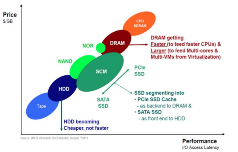
8. 新型存储系统的构成
9. 什么是并行架构
- 并行结构一般是指并行体系结构和软件架构采取并行编程。主要目的是使更多任务或数据同时运行。并行体系结构是指许多指令能同时进行的体系结构;并行编程一般有以下模式:共享内存模式;消息传递模式;数据并行模式。
- 并行计算机是一组处理元素的集合,它们协同快速地解决一些大问题。
10. MIMD 的并行架构包括哪些实现类型
- 对称多处理器:内置多个处理器,共享内存通信,每个处理器运行操作系统的拷贝,例如现在的多核芯片。
- 通过主机的独立 I/O 的非统一共享内存:多处理器,每个都有本地内存,通用可扩展网络,节点上非常轻的 OS 提供简单的服务,调度/同步,用于 I/O 的网络可访问主机。
- 集群:多台独立机接入通用网络,通过消息沟通。
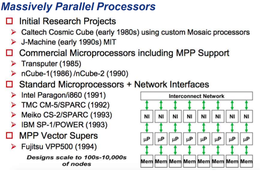
11. MPP 架构的典型例子及主要构成
第三讲:并行编程模型
引入
开头举了许多并行编程的模型的例子:计算$\pi$
历史
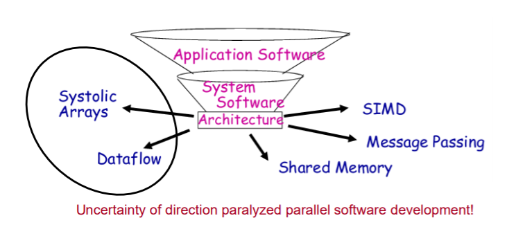
-
1970s – early 1990s,并行机由它的并行模型和语言唯一决定。
Historically (1970s – early 1990s), each parallel machine was unique, along with its programming model and language。
- 架构(Architecture) = 编程模型(prog. model )+ 通信抽象 (comm. abstraction) + 机器(machine);
- 并行架构依附于编程模型(parallel architectures tied to programming models);
-
并行架构发展迅猛:
并行编程模型概述
从并行机器架构中分理出并行编程模型
什么是并行编程模型(感觉 ppt 上没有明确定义)
- 程序员在编码应用程序中所使用的(What programmer uses in coding applications)
-
具体化的通信和同步机制(Specifies communication and synchronization)
- 并行编程模型是作为对硬件和内存架构的抽象而存在的。
并行编程模型的主要包括哪些类型
-
主要的:
-
共享内存(shared address space): openMP
- Independent tasks encapsulating local data
- Tasks interact by exchanging messages
-
消息传递(message passing): MPI
-
Tasks share a common address space
-
任务通过异步读取和写入此空间进行交互(Tasks interact by reading and writing this space asynchronously)
-
-
-
数据并行(data parallel):eg: GPU
- Tasks execute a sequence of independent operations
-
Data usually evenly partitioned across tasks
- Also referred to as 「embarrassingly parallel」
-
其他:
- 数据流(data flow):eg: tensorflow
- (?收缩阵列) systolic arrays
并行编程模型主要包括哪几部分
1. Control 控制
- How is parallelism created?
- In what order should operations take place?
- How are different threads of control synchronized?
2. Naming 变量声明
- What data is private vs. shared?
- How is shared data accessed?
3. Operations 操作
- What operations are atomic?
4. Cost 开销
- How do we account for the cost of operations?
共享内存模型有哪些实现
1.共享内存的定义
Any processor can directly reference any memory location
- Communication occurs implicitly as result of loads and stores
2. 特点
-
便捷性:Convenient
-
Location transparency(位置透明)
-
类似的编程模型,以便在单处理器上进行时间共享
(Similar programming model to time-sharing on uniprocessors)
- Except processes run on different processors
- Good throughput on multiprogrammed workloads
-
-
一般利用进程和线程来是实现
-
读写异步
tasks share a common address space, which they read and write asynchronously。
-
Various mechanisms such as locks / semaphores may be used to control access to the shared memory
-
3. 优缺点(相对于程序员而言)
-
优点
-
An advantage of this model from the programmer’s point of view is that the notion of data 「ownership」 is lacking, so there is no need to specify explicitly the communication of data between tasks。
-
Program development can often be simplified。
-
-
缺点
- 存在数据竞争,难以理解数据的局部性
4. 实现的两种方式
-
单机上,依赖编译器和硬件将程序变量转换成实物理地址,即全局地址。
Native compilers and/or hardware translate user program variables into actual memory addresses, which are global。
-
在分布式系统中,内存物理上分布在同一网络不同机器上,但是通过软件和硬件转换成全局地址。
On distributed shared memory machines, such as the SGI Origin, memory is physically distributed across a network of machines, but made global through specialized hardware and software。
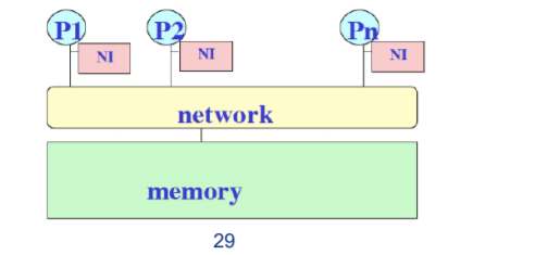
5. 实现的典型架构举例
-
SAS Machine Architecture
-
其中的典型架构:对称多处理器 One representative architecture: SMP
下面是实现原理
-
Used to mean Symmetric MultiProcessor:
All CPUs had equal capabilities in every area, e.g., in terms of I/O as well as memory access
-
Evolved(发展) to mean Shared Memory Processor:
Non-message-passing machines (included crossbar as well as bus based systems 系统总线)
-
Now it tends to refer to bus-based shared memory machines:
Small scale: < 32 processors typically
-
-
-
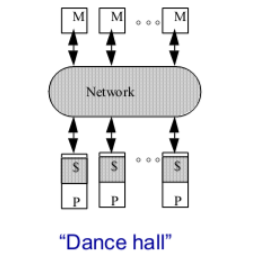
上面的架构在规模一大会出现问题(左图是有问题的初始架构,右边是改进的)
-
左边的问题:
-
互连的总线等成本问题 (Problem is interconnect):
cost (crossbar) or bandwidth (bus)
-
带宽不会提升(Dance-hall: bandwidth is not scalable, but lower cost than crossbar)
- Latencies to memory uniform, but uniformly large
-
-
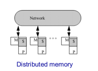
改进成右边:
-
Distributed memory or non-uniform memory access (NUMA):
Construct shared address space out of simple message transactions across a general-purpose network (e.g. read-request, read-response)。
-
共享内存之线程模型
1. 概述
- 最典型的共享内存编程模型
- 单进程可以有多个并发的执行路径
2. 线程的特点
呃……操作系统也学了,不说了
算了还是说一下:
- 含私有变量(栈上的)
- 共享变量(堆上的,静态变量等等)

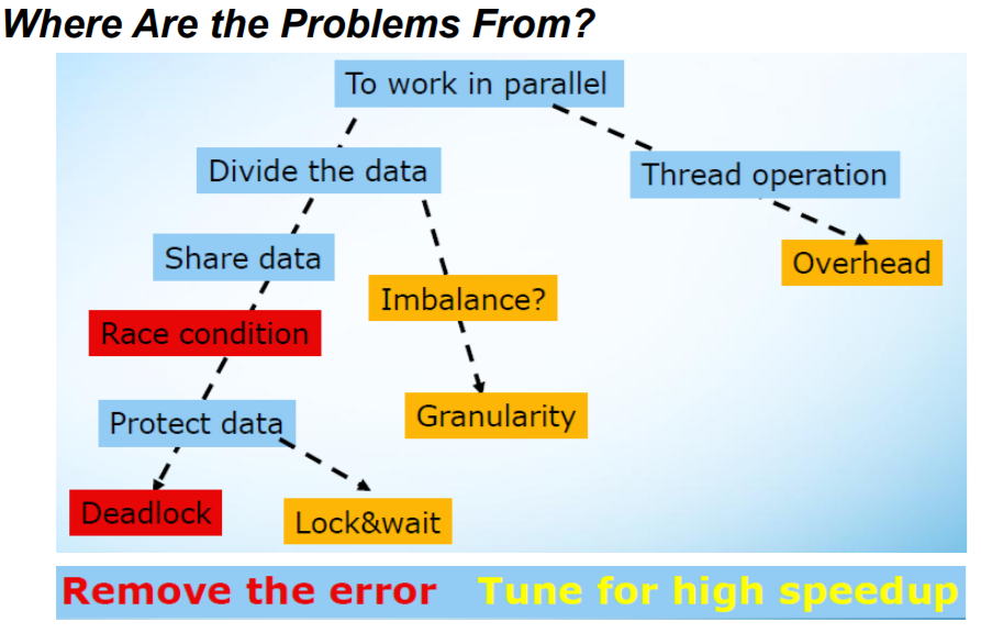
>1 插入内容:造成并行编程模型不能达到理想加速比
-
利用 Amdahl’s Law 定律,分析如下:有的部分不能并行
-
还有其他的问题:
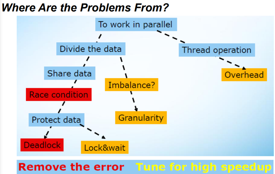
问题出在,一图便知:
- 线程创建需要开销。
- 数据划分会出现不均衡(负载不均衡)。
- 共享数据会出现 RC 问题、死锁问题:加锁、解锁影响性能。
>2. 插入内容:Decomposition(解耦)
有下列两种含义:
- (数据解耦)Data decomposition
- Break the entire dataset into smaller, discrete portions, then process them in parallel
- Folks eat up a cake
- (任务解耦)Task decomposition
- Divide the whole task based on natural set of independent sub-tasks
- Folks play a symphony
注意事项:Considerations
- Cause less or no share data
- Avoid the dependency among sub-tasks, otherwise become pipeline
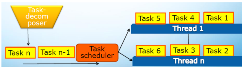
3. 任务(Task)和线程(Thread)之间的关系
任务的特点:
-
任务包含数据和它的进程,任务被调度到线程上进行执行(A task consists the data and its process, and task scheduler will attach it to a thread to be executed)。
- 任务比线程更轻量级 (Task operation is much cheaper than threading operation)。
- 线程之间可以通过任务的 steal 达到负载均衡的目的(Ease to balance workload among threads by stealing)。
- 任务适合多种数据结构:Suit for list, tree, map data structure
任务有静态调度和动态调度。
4. 什么是线程竞争?如何解决
额…RC 问题,还不知道吗?那操作系统挂定了…
RC 问题
-
定义:
一般来说,指的是多个线程在同一时间访问同样的内存位置,其中至少有一个线程进行写操作。
-
解决:
- 设置临界区:(Control shared access with critical regions)
- Mutual exclusion and synchronization, critical session, atomic
- 把全局变量变成线程的局部变量( Scope variables to be local to threads)
- Have a local copy for shared data
- Allocate variables on thread stack
- 设置临界区:(Control shared access with critical regions)
死锁
-
定义:
2 or more threads wait for each other to release a resource。
-
解决:
- Always lock and un-lock in the same order, and avoid hierarchies if possible
- Use atomic
1. 什么是并行编程模型
- 并行编程模型是并行计算机体系架构的一种抽象,它便于编程人员在程序中编写算法及其组合。(百度)
- 历史上(70 年代至 90 年代初),每台并行机都是独一无二的,其编程模型和语言也是独一无二的。架构=程序模型+通信抽象+机器,并行架构与编程模型相关。
- 现在,我们将编程模型与底层的并行机器体系结构分离开来。
- 主要编程模型有:共享地址空间、消息传递、数据并行;其他类型有:数据流、收缩阵列。
- 通过扩展「计算机体系结构」以支持通信与合作。旧:指令集架构;新:通信架构。
- 定义:关键抽象、边界和接口;实现接口的组织结构。
- 编译器、库和操作系统是重要的桥梁。
2. 并行编程模型主要包括哪些类型,主要特点是什么
- 程序员在编码应用程序中使用什么来指定通信和同步
- 多道程序设计:无通信或同步,在程序级别
- 共享地址空间:如公告板
- 消息传递:如信件或电话,明确的点到点
- 数据并行:对数据进行更严格的全局操作,使用共享地址空间或消息传递实现
- 并行编程模型及特点
- 消息传递(message passing):封装本地数据的独立任务,任务通过交换消息进行交互。
- 共享内存(shared memroy):任务共享公用地址空间,任务通过异步读写此空间进行交互。
- 数据并行化(data parallelization):任务执行一系列独立的操作,数据通常在任务之间均匀分区,也被称为「令人尴尬的并行」。
3. 并行编程模型主要包括哪几部分
- 控制:如何创建并行性;应按什么顺序进行操作;不同的控制线程是如何同步的
- 命名:什么数据是私有的还是共享的;如何访问共享数据
- 操作:什么操作是原子操作
- 成本:我们如何计算运营成本
4. 共享内存模型有哪些实现
- 共享内存模型
- 任何处理器都可以直接引用任何内存位置,由于加载和存储而隐式发生通信;方便;位置透明度;与单处理器时间共享类似的编程模型。
- 在这个编程模型中,任务共享一个公共地址空间,它们异步读写。可以使用各种机制,如锁/信号灯来控制对共享内存的访问。从程序员的角度来看,该模型的一个优点是缺乏数据「所有权」的概念,因此无需明确规定任务之间的数据通信。程序开发通常可以简化。在性能方面的一个重要缺点是,越来越难以理解和管理数据位置。将数据保持在处理器的本地,这样可以节省在多个处理器使用相同数据时发生的内存访问、缓存刷新和总线流量。不幸的是,控制数据位置很难理解,并且超出了普通用户的控制范围。
- 实现
- SAS Machine Architecture
- Scaling Up
5. 造成并行编程模型不能达到理想加速比的原因
6. 任务和线程之间的关系
- 分解
- 数据分解:将整个数据集分解为更小、离散的部分,然后并行处理它们
- 任务分解:根据独立子任务的自然集合划分整个任务
- 任务和线程
- 任务由数据及其进程组成,任务调度程序会将其附加到要执行的线程上。
- 任务操作比线程操作便宜得多。
- 通过窃取轻松平衡线程之间的工作量。
- 任务适合列表、树、地图数据结构
- 注意事项
任务比线程多
- 更灵活地安排任务
- 轻松平衡工作量
任务中的计算量必须足够大,以抵消管理任务和线程的开销。
静态调度
任务是独立函数调用的集合,或者是循环迭代
动态调度
任务执行长度可变且不可预测 可能需要一个额外的线程来管理共享结构以保存所有任务
7. 什么是线程竞争,如何解决
- 竞争
- 线程之间「竞争」以获取资源;执行令被假定,但不能保证;存储冲突最常见;多个线程并发访问同一内存位置,至少有一个线程正在写入;可能在任何时候都不明显
- 注意事项:互斥和同步、临界区、原子操作
- 死锁
- 两个或多个线程等待彼此释放资源;一个线程等待一个永远不会发生的事件,比如挂起的锁。
- 注意事项:始终按相同顺序锁定和解除锁定,并尽可能避免层次结构;使用原子操作
- 线程安全例程/库
- 它在多个线程同时执行期间正常工作。
- 非线程安全标志 访问全局/静态变量或堆 分配/重新分配/释放具有全局范围(文件)的资源 通过句柄和指针间接访问
- 注意事项
任何更改的变量必须是每个线程的本地变量 例程可以使用互斥来避免与其他线程冲突
- 工作量不平衡
- 所有线程以相同的方式处理数据,但一个线程分配了更多的工作,因此需要更多的时间来完成它并影响整体性能。
- 注意事项
使内环平行
向细粒倾斜 选择合适的算法 分而治之,master and work, work-stealing
- 粒度
- 较大实体的细分程度,粗粒意味着越来越少的成分,细粒度意味着越来越小的成分
- 注意事项:细粒度将增加任务调度程序的工作量;粗粒度可能导致工作负载不平衡;设定适当粒度的基准
- 锁和等待
- 保护共享数据并确保任务按正确顺序执行,使用不当会产生副作用
- 注意事项
选择适当的同步原语 使用非锁定锁 降低锁粒度 不要做一个锁中心 为共享数据引入并发容器
第四讲:并行编程方法论
什么是增量式并行化
- Study a sequential program (or code segment)
- Look for bottlenecks & opportunities for parallelism
- Try to keep all processors busy doing useful work
Culler 并行设计流程
主要分四个步骤:(Decomposition)解耦、(Assignment)分派、(Orchestration)配置、(mapping)映射。
图解如下:
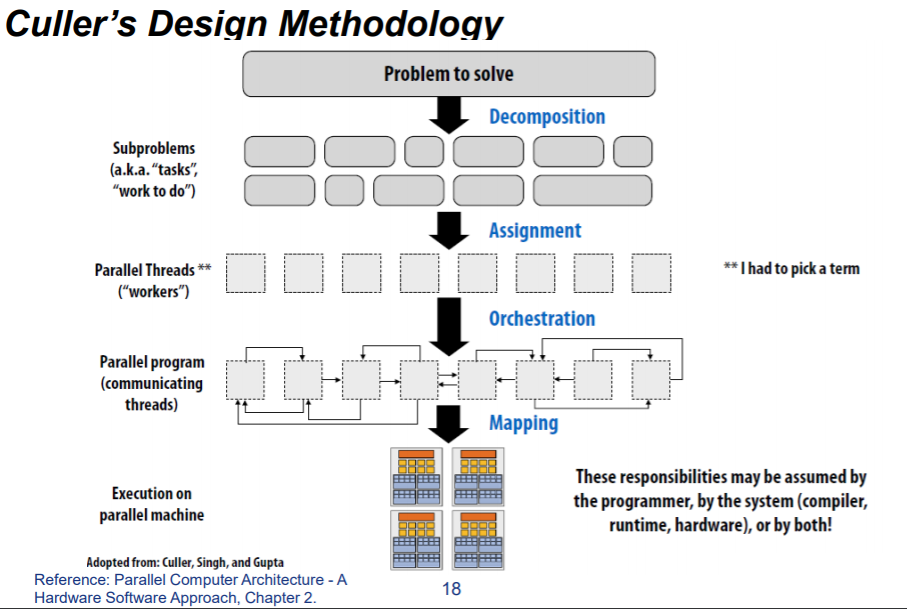
1. Decomposition
定义
Break up problem into tasks that can be carried out in parallel.
- Decomposition need not happen statically
- New tasks can be identified as program executes
核心思想、目的
创建最少任务且使得所有的机器上的执行单元都处于忙碌状态
关键方面
识别出依赖部分。(identifying dependencies)
负责的对象
一般是程序员来做这件事情。
2. Assignment
定义
分发任务给线程。
目标
负载均衡,减少通信开销。
特点
静态动态皆可,一般需要程序员来负责,也有非常多语言可以自动对此负责。
3. Orchestration(配置)
定义
- 结构化通信(Structuring communication)
- 增加同步来保证必要的依赖性(Adding synchronization to preserve dependencies if necessary)
- 在内存中组织数据结构
- 调度任务
目的
减少通信和同步的开销,保护数据的局部性,减少额外开销(overhead).
4. Mapping
定义
Mapping 「threads” to hardware execution units.
执行对象
- OS
- compiler
- hardware
Foster 并行设计流程
分为四个部分:
- Partitioning
- Communication
- Agglomeration (归并、组合)
- Mapping。
图解:
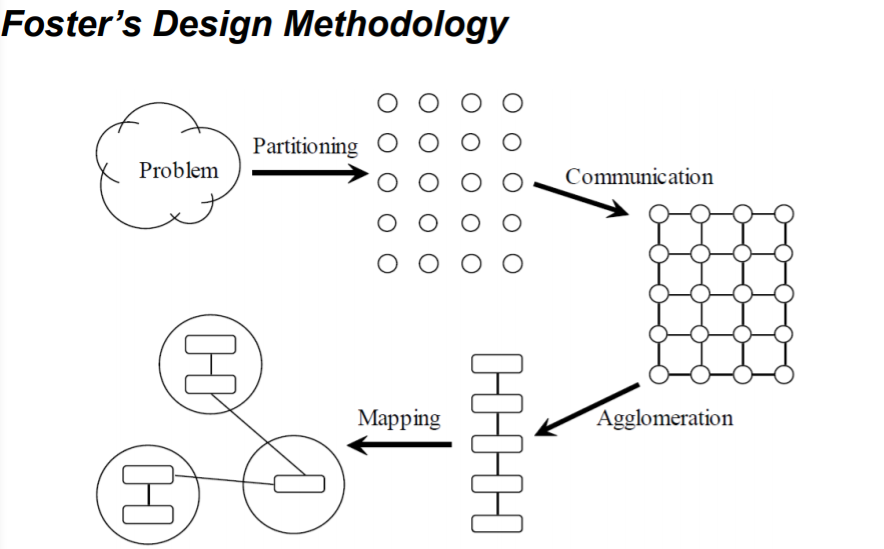
1. 分解
定义
Dividing computation and data into pieces
三种不同实现方式及目的
Exploit data parallelism(实现数据并行)
- (Data/domain partitioning/decomposition)
- Divide data into pieces
- Determine how to associate computations with the data
Exploit task parallelism(实现任务并行)
- (Task/functional partitioning/decomposition)
- Divide computation into pieces
- Determine how to associate data with the computations
Exploit pipeline parallelism(实现流水并行)
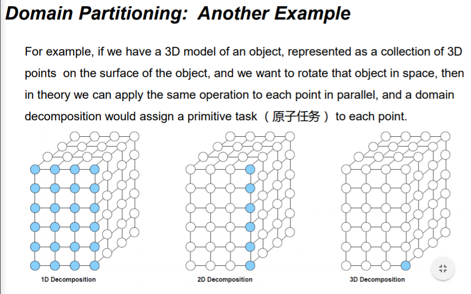
方式之一: Domain Partitioning (按域 / 数据分解)
过程
- (数据如何划分给处理器)First, decide how data elements should be divided among processors
- (每个处理器如何执行任务)Second, decide which tasks each processor should be doing
举例
- Find the largest element of an array.
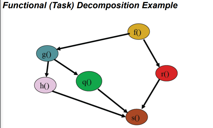
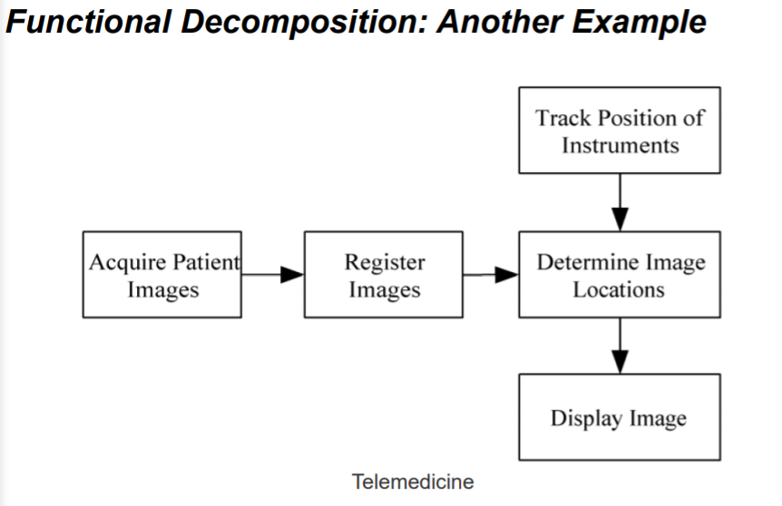
方式之二:Functional (Task) Decomposition
过程
- (划分任务给处理器)First, divide tasks among processors
- (再确定数据的获取)Second, decide which data elements are going to be accessed (read and/or written) by which processor
举例
-
event-handler for GUI
-
another eg:
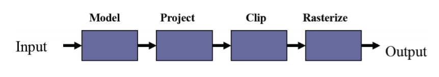
方式之三:Pipelining
过程
- Special kind of task decomposition
- 「Assembly line」 parallelism
举例
-
3D rendering in computer graphics
分解注意的问题
- At least 10x more primitive tasks than processors in target computer
- If not, later design options may be too constrained
- Minimize redundant computations and redundant data storage
- If not, the design may not work well when the size of the problem increases
- Primitive tasks roughly the same size
- If not, it may be hard to balance work among the processors
- Number of tasks is an increasing function of problem size
- If not, it may be impossible to use more processors to solve large problem instances
2. 通信 Communication
定义:
Determine values passed among tasks
- Task-channel graph(任务数据依赖图)
分类:
- (局部通信)Local communication
- Task needs values from a small number of other tasks
- Create channels illustrating data flow
- (全局通信)Global communication
- Significant number of tasks contribute data to perform a computation
- Don’t create channels for them early in design
注意事项
- Communication is the overhead of a parallel algorithm, we need to minimize it
- Communication operations balanced among tasks
- Each task communicates with only small group of neighbors
- Tasks can perform communications concurrently
- Task can perform computations concurrently
3. Agglomeration (整合、归并)
定义
Grouping tasks into larger tasks(小任务变大任务)
目标和意义
-
(提升性能)Improve performance:
- (减少通信)Eliminate communication between primitive tasks agglomerated into consolidated task.
- 比如:Combine groups of sending and receiving tasks
-
(保持问题的可并行性)Maintain scalability of program:
举例:
- Suppose we want to develop a parallel program that manipulates a 3D matrix of size 8 x 128 x 256.
- If we agglomerate the second and third dimensions, we will not be able to port the program to a parallel computer with more than 8 CPUs.
-
(简化编程)Simplify programming (reduce software engineering costs):
- If we are parallelizing a sequential program, one agglomeration may allow us to make greater use of the existing sequential code, reducing the time and expense of developing the parallel program.
在消息传递型的编程模型中:In message-passing programming, goal often to create one agglomerated task per processor.
4. Mapping(映射)
定义
把任务分配到处理器上的过程:Process of assigning tasks to processors
- Centralized multiprocessor(中心多处理器系统): mapping done by operating system
- Distributed memory system(分布式系统): mapping done by user
目标矛盾
- Maximize processor utilization(最大化处理器利用率)
- Minimize interprocessor communication(最小化通信)
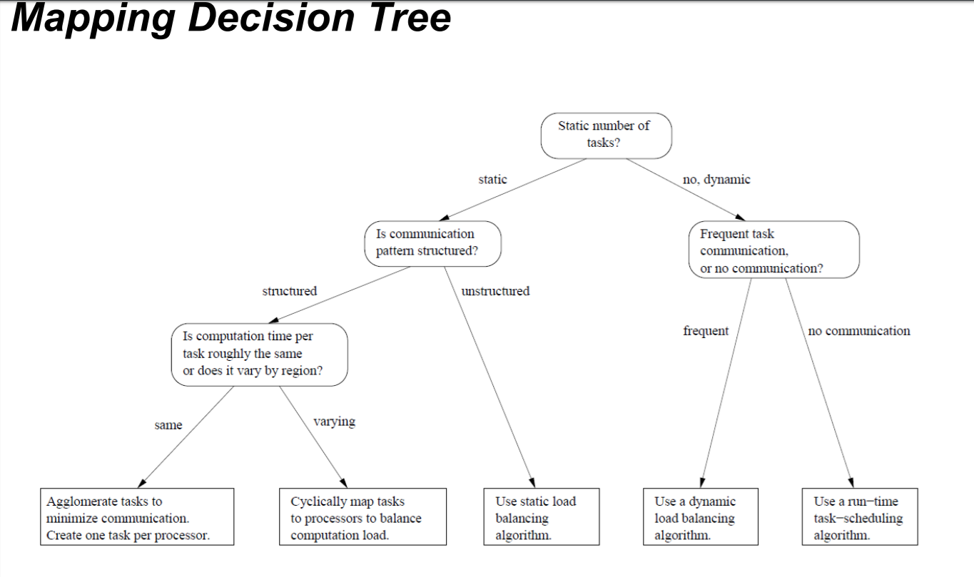
决策(树)
分两种情况:静态任务和动态任务
-
静态任务(Static number of tasks)
-
Structured communication(有解构的通信)
-
Constant computation time per task
(a) Agglomerate tasks to minimize communication (b) Create one task per processor
-
Variable computation time per task
(a) Cyclically map tasks to processors
-
-
Unstructured communication(无结构的通信)
- 使用动态负载均衡算法 Use a static load balancing algorithm
-
-
动态任务(Dynamic number of tasks)
- Frequent communications between tasks
- 动态负载均衡算法 Use a dynamic load balancing algorithm
- Many short-lived tasks
- 运行时调度算法 Use a runtime task-scheduling algorithm
- Frequent communications between tasks
决策树如下:
并行设计举例——边界值-散热问题
第四讲:并行编程方法论,内容要点
-
什么是增量式并行化? Study a sequential program (or code segment) 研究串行程序(代码段) Look for bottlenecks & opportunities for parallelism 寻找并行性的瓶颈和机会 Try to keep all processors busy doing useful work 尽量让所有的处理器做有用的工作
-
Culler 并行设计流程?
-
Foster 并行设计流程? Partitioning(划分) communication(通信) Agglomeration(归并,组合) mapping(聚合)
-
按数据分解和按任务分解的特点? Exploit data parallelism 利用数据并行性 (Data/domain partitioning/decomposition) Divide data into pieces 将数据分成几部分 Determine how to associate computations with the data 确定如何将计算与数据相关联
Exploit task parallelism 利用任务并行性 (Task/functional partitioning/decomposition) Divide computation into pieces 将计算任务分成几部分 Determine how to associate data with the computations 确定如何将数据与计算关联
-
并行任务分解过程中应该注意的问题有哪些? First, divide tasks among processors Second, decide which data elements are going to be accessed (read and/or written) by which processor
-
整合的意义是什么? Improve performance 提高性能 Maintain scalability of program 保持程序的可扩展性 Simplify programming (reduce soft ware engineering costs) 简化编程(降低软件成本)
- Mapping(映射)如何决策?
- 熟悉一些并行设计的例子。
第五讲:OpenMP 并行编程模型,内容要点
什么是 OpenMP
- 提供针对共享式内存并行编程的 API
- 简化了并行编程在 fortran、C、C++等环境下
short version:Open Multi-Processing 开放多处理过程 long version: Open specifications for Multi-Processing via collaborative work between interested parties from the hardware and software industry, government and academia
OpenMP is an explicit (not automatic) programming model, offering the programmer full control over parallelization 一种显式(非自动)编程模型,为程序员提供对并行化程序的控制
OpenMP 的主要特点是什么
- OpenMP 通过完全使用线程来实现并行
- 共享内存的编程模型,线程通信主要通过共享内存变量
- 也是因为共享变量可能会导致数据竞争,循环依赖等
OpenMP programs accomplish parallelism exclusively (仅仅) through the use of threads 通过对线程的使用来完成程序的并行化
熟悉 OpenMP 的关键指令
1
2
3
4
5
6
#pragma omp parallel // 表明之后的结构化代码块被多个线程处理
#pragma omp parallel num_threads(thread_count) // 可自定义线程数量
omp_get_thread_num
omp_get_num_threads
#pragma omp critical // 只有一个线程能够执行对应代码块,并且第一个线程完成操作前,没有其他的线程能够开始执行这段代码
#pragma omp parallel for // parallel for 指令生成一组线程来执行后面的结构化代码块(必须是for循环)。
- 一些 OpenMP 常用函数
- omp_get_thread_num() 获取当前线程编号
- omp_get_num_threads() 获取当前线程组的线程数量
- omp_set_num_threads() 设置线程数量
-
所有的 OpenMP 指令都有#pragma omp
[clause, ...]这种形式 - #pragma omp parallel
- 最基本的 parallel 指令,这条 OpenMP 指令后的一段代码将被并行化,线程数量将由系统自行决定,当然我们可以指定线程数量只需要在 parallel 之后加上子句限定即可,num_threads 子句
- #paragm omp parallel num_threads (thread_count),指定我们的并行化代码将由 thread_count 个线程来进行执行
- 介绍一下这个程序运行到这个子句之后的操作,首先程序本身只含有一个线程,在遇到该指令之后,原来的线程继续执行,另外的 thread_count – 1 个线程被启动,这 thread_count 个线程称为一个线程组,原始线程为主线程,额外的 thread_count – 1 个线程为从线程,在并行化代码块的末尾存在一个隐式路障,所有线程都到达隐式路障后从线程结束,主线程继续执行。也就是下图所示的 fork-join 过程
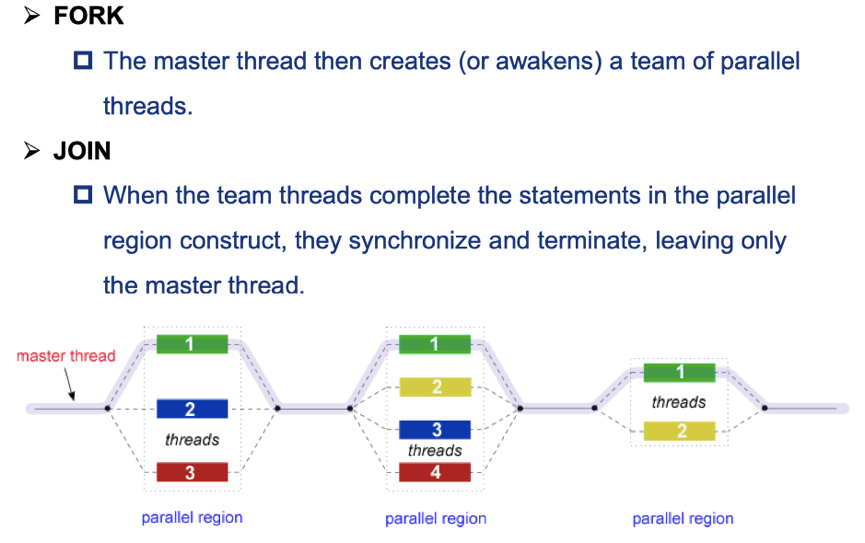
- 介绍一下这个程序运行到这个子句之后的操作,首先程序本身只含有一个线程,在遇到该指令之后,原来的线程继续执行,另外的 thread_count – 1 个线程被启动,这 thread_count 个线程称为一个线程组,原始线程为主线程,额外的 thread_count – 1 个线程为从线程,在并行化代码块的末尾存在一个隐式路障,所有线程都到达隐式路障后从线程结束,主线程继续执行。也就是下图所示的 fork-join 过程
- #pragma omp parallel for
- parallel for 指令,用于并行化 for 循环,这个指令存在以下限制:
- 不能并行化 while 等其他循环。
- 循环变量必须在循环开始执行前就已经明确,不能为无限循环。
- 不能存在其他循环出口,即不能存在 break、exit、return 等中途跳出循环的语句。
- 在程序执行到该指令时,系统分配一定数量的线程,每个线程拥有自己的循环变量,互不影响,即使在代码中循环变量被声明为共享变量,在该指令中,编译过程仍然会为每一个线程创建一个私有副本这样防止循环变量出现数据依赖,跟在这条指令之后的代码块的末尾存在隐式路障。
- parallel for 指令,用于并行化 for 循环,这个指令存在以下限制:
-
private
-
private 子句可以解决私有变量的问题,一些共享变量在循环中,如果每个线程都可以访问的话,可能会出错,该子句就是为每个线程创建一个共享变量的私有副本解决循环依赖,如下所示。注 private 的括号中可以放置多个变量,逗号分隔
-
private_emaxple.c
#pragma omp parallel for private (x) for (i = 0; i <= 10;i++) { x = i; printf("Thread number: %d x: %d\n",omp_get_thread_num(),x); }- 关于私有变量还有一下几点 1. 每一个线程都含有自己的私有变量副本 2. 所有线程在 for 循环中不能访问最开始定义的那个全局变量,它们操作的都是自己的私有副本
-
- firstprivate
- 告诉编译器,每个线程的私有副本初始化为共享变量的值,只是在每个线程开始执行并行代码块时就分配给私有副本的而不是每次循环迭代分配一次
-
firstprivete.c
int x = 44;
#pragma omp  parallel for firstprivate (x)
for (i=0;i<=1;i++) {
  //x = i;
  printf("Thread number: %d  x: %d\n",omp_get_thread_num(),x);
}
printf("x is %d\n", x);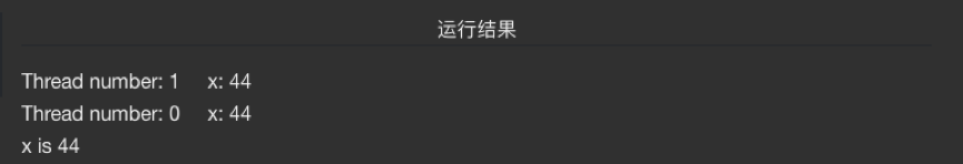
-
lastprivate
-
告诉编译器,将最后一个离开并行化块的线程的最后一次循环迭代的私有副本赋值给原先的共享变量
-
lastprivate.c
int x = 44;
#pragma omp  parallel for lastprivate (x)
for (i = 0;i <= 1;i++) {
    x = i;
    printf("Thread number: %d    x: %d\n",omp_get_thread_num(),x);
}
printf("x is %d\n", x);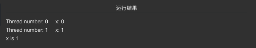
-
- single
- 最先到达的线程执行该子句后面的代码块,其余不执行这个代码块的线程会在代码块的末尾被阻塞(隐式 barriers),等待所有的线程执行到该位置后,继续向后执行,如果在 single 后加上 nowait 指令,则不执行这个代码块的线程不需要等待,继续向后执行
-
master
- 该子句仅有主线程执行后面的代码块,其他线程直接跳过该子句后面的代码块,且不存在隐式 barriers
-
sections
- #pragma omp sections 在这条指令后的代码块进行串行执行
-
#pragma omp parallel sections 在这条指令后的代码块才是进行并行执行,里面每一个 section 都只需要一个线程去执行,当然如果一个线程足够快允许实现,他可以执行多个 section
-
sections.c
   #pragma omp  sections
    {
        #pragma omp section
        {
            printf("section0,threadid=%d\n",omp_get_thread_num());
            sleep(1);
        }
        #pragma omp section
        {
            printf("section1,threadid=%d\n",omp_get_thread_num());
            sleep(1);
        }
        #pragma omp section
        {
            printf("section2,threadid=%d\n",omp_get_thread_num());
            sleep(1);
        }
    }

    #pragma omp parallel sections num_threads(4)
    {
        #pragma omp section
        {
            printf("section3,threadid=%d\n",omp_get_thread_num());
            sleep(1);
        }
        #pragma omp section
        {
            printf("section4,threadid=%d\n",omp_get_thread_num());
            sleep(1);
        }
        #pragma omp section
        {
            printf("section5,threadid=%d\n",omp_get_thread_num());
            sleep(1);
        }
    }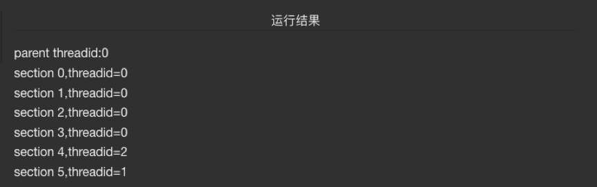
-
reduction
- 规约子句
#pragma omp ……reduction<opreation : variable list>-
opreation +、-、* 、& 、| 、&& 、|| 、^ 将每个线程中的变量进行规约操作例如 #pragma omp ……reduction<+ : total>就是将每个线程中的 result 变量的值相加,最后在所有从线程结束后,放入共享变量中,其实这也可以看作是 private 子句的升级版,下面的例子,最后共享的 total 中存入就是正确的值(浮点数数组数字之和),其他操作符的情况可以类比得到
-
reduction.c
float total = 0.;

#pragma omp parallel for reduction(+:total)
for (size_t i = 0; i < n; i++) {
    total += a[i];
}
return total;
-
- #pragma omp parallel
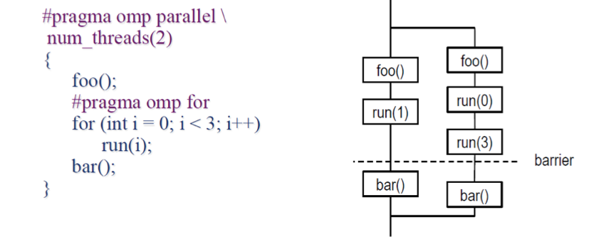
熟悉 OpenMP 关键指令的执行过程
- 观察下图中的执行顺序
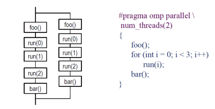
- 图中的虚线路障是 parallel for 模块所带的隐式路障
第六讲:OpenMP 中的竞争和同步,内容要点
OpenMP 中为了保证程序正确性而采用哪些机制
barriers(障碍,屏障) memory fence(内存屏障) mutual exclusion(互斥)
什么是同步,同步的主要方式有哪些
The process of managing shared resources so that reads and writes occur in the correct order regardless of how the threads are scheduled 用户进程共享资源让读和写的操作以正确的顺序发生,无论线程是如何安排。
barriers mutual exclusion pthread_mutex_lock
- 管理共享资源的过程,不论线程调度顺序如何,读取和写入资源都可以按照正确的发生
- 方法:barrier、互斥锁、信号量
OpenMP Barrier 的执行原理
A synchronization point at which every member in a team of threads must arrive before any member can proceed
- ⼀个同步点,线程团队中的每个成员必须在任何成员继续之前到达该同步点,也就是在还有其他线程未到达时,每个线程都将被阻塞
- 注:parallel for 和 single 都有隐式的 barriers,在它们的代码块结尾的地方,可使用 nowait 禁用掉这个隐式的 barriers
OpenMP 中竞争的例子
1
2
3
4
5
6
7
8
double area, pni, x;
int i, n;
area = 0.0;
for (i = 0; i <n; i++) {
x = (i + 0.5)/n;
area += 4.0/(1.0 + x*x);
}
pi = area / n;
如果两个线程同时执行 area += 4.0/(1.0 + x*x);可能会在一个线程更新 area 的值之前另一个线程就对 area 进行读操作
1
2
3
4
5
6
7
8
9
10
11
12
13
- 这个for循环的并行会导致竞争的发生,原因是因为多个线程对同一个共享变量访问时间的非确定性导致结果可能出错,多个线程访问area += 4.0 / (1.0 + x*x)就可能导致竞争
```C
    double area, pni, x;
    int i, n;
    ...
    area = 0.0;
    #pragma omp for
    for (i = 0; i <n; i++) {
        x = (i + 0.5)/n;
        area += 4.0/(1.0 + x*x);
    }
    pi = area / n;
```
OpenMP 中避免数据竞争的方式有哪些
Scope variables to be private to threads 设置线程专用的范围变量 如: Use OpenMPprivate clause 使用 openmpprivate 子句 Variables declared within threaded functions 在线程函数中申明变量 Allocate on thread’s stack (pass as parameter) 在线程堆栈上分配(作为参数传递)
Control shared access with critical region 控制关键区域的共享访问 如: Mutual exclusion and synchronization 互斥和同步
1
2
3
4
5
6
7
8
9
10
- 1. 变量私有化
    - 使用OpenMP的private子句将变量变为私有
    - 在线程函数内声明变量,这样变量将属于这个线程
    - 在线程堆栈上进行分配

- 2、将共享变量放置进入临界区

-   3、互斥访问
    - 信号量
    - 互斥锁机制
OpenMP Critical 与 Atomic 的主要区别是什么
Critical 确保一次只有一个线程执行结构化代码。
atomic 只能用在形如 x
1
2
3
4
5
6
7
8
9
10
11
12
13
14
15
16
17
18
19
20
21
22
23
24
25
26
27
28
29
30
31
32
33
- #pragma omp critical该指令保护了
    1、WorkOne(i)的调用过程,也就是在WorkOne(i)函数内部也是临界区
    2、从内存中找到index[i]值的过程
    3、将WorkOne(i)的值加到index[i]的过程
    4、将内存中index[i]更新的过程
    后面跟的语句相当于串行执行
    ```C
    #pragma omp parallel for
    {
        for(int i = 0; i < n; i++) {
            #pragma omp critical
            x[index[i]] += WorkOne(i);
            y[i] += WorkTwo(i);
        }
    }
    ```

- Atomic指令只对一条指令形成临界区,而且语句的格式收到限制
    1、将WorkOne(i)的值加到index[i]
    2、更新内存中index[i]的值
    只将单一一条语句设置为临界区
    如果不同线程的index[i]非冲突的话仍然可以并行完成
    只有当两个线程的index[i]相等时才会触发使得这两个线程排队执行这条语句
    ```C
    #pragma omp parallel for
    {
        for(int i = 0; i < n; i++) {
            #pragma omp atomic
            x[index[i]] += WorkOne(i);
            y[i] += WorkTwo(i);
        }
    }
    ```
第七讲:OpenMP 性能优化,内容要点
什么是计算效率
核心利用率的衡量标准,计算公式为加速比/核心数
加速比:Speedup = 串行执行时间/并行执行时间
Efficiency(效率)
- A measure of core utilization
- Speedup divided by the number of cores
核心利用率的一种度量 - Efficiency = Speedup/nums of cores
调整后的 Amdahl 定律如何理解
- 原来的 Amdahl 定律过于乐观
- 忽略了并行处理的开销,如创建/终止线程。而并行处理开销一般是关于线程数(核心 数)的增函数。
- 忽略了计算量难以均衡地分配到每个核心上,负载不均衡以及核心等待时间都是一种开销。
- 改进后的 Amdahl 定律
1
2
3
4
5
6
7
8
9
10
11
12
13
14
    n       问题规模
    p       核心数
    S(n,p)  问题的加速比
    Ts(n)   串行部分的时间花费
    Tp(n)   并行部分的时间花费
    Tr(n,p) 并行开销

    S(n,p)<=( Ts(n)+Tp(n) )/( Ts(n)+Tp(n)/p+Tr(n,p) )

    最大加速比:
    Tp(n)/p:假设并行计算部分可以在核心完美分配
    Tr(n,p)趋向于0

    加速比是关于问题规模的递增函数
1
2
3
4
5
6
7
8
9
10
11
12
13
14
15
16
17
- Amdahl太过乐观,很多并行处理开销并没有考虑
1. 创建和终止线程所花费的时间,这是多线程并行的必须开销。
2. 工作量在核心之间平均分配,但是在实际运行时,这并不成立,先执行完任务的核心等待时间是另一种形式的开销,即所谓的负载不均衡。
- 所以进行Amdahl公式的改进,加上线程开销部分, 为了获得最大的加速比,我们就需要将并行开销尽可能减小,同时使用更多的核,改进后的公式如下所示
$\psi(n,p) \leq \frac{\sigma(n) + \varphi(n)}{\sigma(n) + \frac{\varphi(n)}{p} + \kappa(n,p)}$
n - 问题规模
p - 核心数
$\psi(n,p)$ - 在问题规模为n核心数为p的情况下并行的加速比
$\sigma(n)$ - 代码串行部分执行时间
$\varphi(n)$ - 代码并行部分执行时间
$\kappa(n,p)$ - 并行开销
- 如下图表示当我们的问题规模达到一定程度后,并行程序的加速比主要由并行部分来决定,因为随着问题规模的增加,程序串行部分也会逐渐较少,同时并行部分将占据主要时间,可以忽略掉串行时间的影响,加速比主要由并行部分决定


OpenMP 中 Loop 调度的几种方式,执行过程
1. Static schedule
- 循环执行前把迭代分配给线程
-
schedule (static [, chunk])
- Blocks of iterations of size 「chunk」 to threads
每个分配给线程的迭代块的计算量「大致相当」\ - Round robin distribution
轮循分配 T1,T2,T3,T1,T2,T3…… - Low overhead, may cause load imbalance
低开销,但可能会负载不平衡
- Blocks of iterations of size 「chunk」 to threads
- 适用于可预见和简单的循环
2. Dynamic schedule
- 循环的执行期间把迭代分配给线程
- schedule (dynamic [, chunk])
- Threads grab 「chunk」 iterations
线程获取任务块 - When done with iterations, thread requests next set
当迭代完成后,请求下一组任务 - Higher threading overhead, can reduce load imbalance
较高的线程开销,但可以做到负载均衡
- Threads grab 「chunk」 iterations
- 适用于不可预知或高度可变的循环
3. Guided schedule
- 调度顺序以及任务块大小,如:T1(1 block),T2(0.5 block),T3(0.25 Block),T3(0.125 block)……
- schedule (guided [, chunk])
- Dynamic schedule starting with large block
以较大的任务块开始动态调度 - Size of the blocks shrink; no smaller than 「chunk」
任务块大小减小,但任务块大小有下界 - The initial block is proportional to
开始时块大小- number_of_iterations / number_of_threads
总任务/线程数
- number_of_iterations / number_of_threads
- Subsequent blocks are proportional to
后续块大小- number_of_iterations_remaining / number_of_threads
当前任务/线程数
- number_of_iterations_remaining / number_of_threads
- Dynamic schedule starting with large block
-
最好用作动态的特殊情况,以在计算越来越耗时的情况下减少调度开销
-
OpenMP 的调度方案,影响着循环迭代映射到线程的方式 动态调度:在执行循环期间分配线程的迭代次数 静态调度:在执行循环前分配线程的迭代次数
-
shedule(type[ , chunksize])子句是进行循环调度的指令
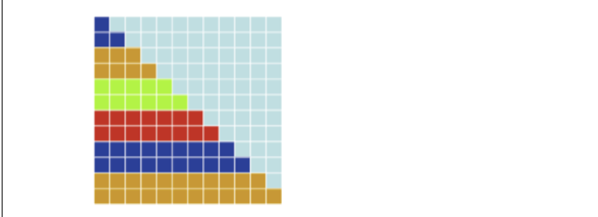
- shedule(static [, chunksize])
- 这是静态调度,每个线程都将分到 chunksize 个循环迭代,可能存在负载不均衡
#pragma omp parallel for shedule(static, 2)
for(int i = 0; i < 12; i++) {
  for(int j = 0; j <= i; j++) {
  a[i][j] = ......
  }
}
其具体分配如下,同一种颜色代表分配给同一个线程的任务
- 这是静态调度,每个线程都将分到 chunksize 个循环迭代,可能存在负载不均衡
- shedule(dynamic [, chunksize])
- 这是动态调度方案,每个循环开始都将分到一份chunksize个循环迭代的块,之后执行完这个块后的线程请求另外一块chunksize大小的迭代继续执行,这个调度方案就可以解决负载不均衡的问题,适用于不可预测和变化较大的工作
 #pragma omp parallel for shedule(dynamic, 2)
 for(int i = 0; i < 12; i++) {
  for(int j = 0; j <= i; j++) {
  a[i][j] = ......
  }
 }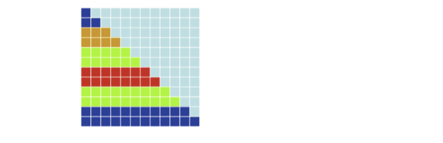
- 这是动态调度方案,每个循环开始都将分到一份chunksize个循环迭代的块,之后执行完这个块后的线程请求另外一块chunksize大小的迭代继续执行,这个调度方案就可以解决负载不均衡的问题,适用于不可预测和变化较大的工作
- shedule(guided [, chunksize])
- guided调度和dynamic调度很相似,唯一不同之处就是块的大小在不断的进行变化,每次需要分配时都重新计算需要划分的循环迭代的数目,公式为 剩余的循环迭代总数 / 线程总数(取整)
- 该种调度方式最好⽤作动态的特殊情况,以便在计算逐渐耗费时间时减少调度开销
 #pragma omp parallel for shedule(guided)
 for(int i = 0; i < 12; i++) {
     for(int j = 0; j <= i; j++) {
     a[i][j] = ......
     }
 }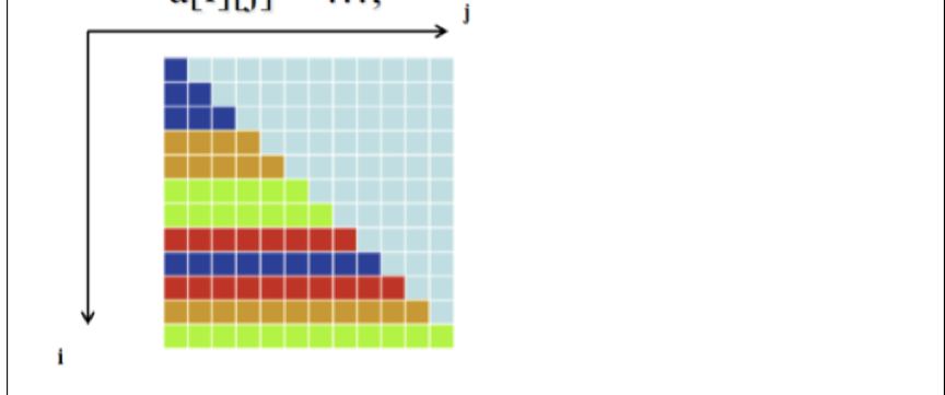
-
OpenMP 中 Loop 转换的方式包括哪几种?熟练掌握
1. Loop fission——循环拆分
- Begin with single loop having loop-carried dependence
从具有循环依赖的单循环开始 - Split loop into two or more loops
把循环拆成两个或多个循环 - New loops can be executed in parallel
新的循环可以并行执行
2. Loop fusion——循环合并
- The opposite of loop fission
与循环拆分相反 - Combine loops increase grain size
合并循环以增加粒度 - Loop Fusion with Replicated Work
循环合并和操作转换(改变操作使得结果相同但更简单)- Every thread iteration has a cost
每个线程的迭代是有开销的 - Example: Barrier synchronization
比如:同步时使用的 barrier - Sometimes it’s faster for threads to replicate work than to go through a barrier synchronization
有时候,改变操作以避免 barrier 是要执行得更快
- Every thread iteration has a cost
3. Loop exchange(Inversion)——循环交换(反转)
- Nested for loops may have data dependences that prevent parallelization
嵌套 for 循环可能具有阻止并行化的数据依赖关系 -
Exchanging the nesting of for loops may
交换的嵌套 for 循环可以- Expose a parallelizable loop
使循环可以并行 - Increase grain size
提高操作粒度 -
Improve parallel program’s locality
提高并行程序的局部性- Loop fission
- 将原来存在循环依赖的循环进行划分,划分成两个或者多个可以完全并行执行的循环
- 划分前
float *a, *b; ...... for(int i = 0; i < N; i++) { //perfectly parallel if(b[i] > 0.0) a[i] = 2.0; else a[i] = 2.0 * fabs(b[i]); //loop-carried dependence b[i] = a[i - 1]; } - 划分后
float *a, *b;
......
#pragma omp parallel
{
#pragma omp for
for(int i = 0; i < N; i++) {
  //perfectly parallel
  if(b[i] > 0.0) a[i] = 2.0;
  else a[i] = 2.0 * fabs(b[i]);
  //loop-carried dependence
}
#pragma omp for
for(int i = 0; i < N; i++) b[i] = a[i - 1];
}
-
Loop fusion
- 将不存在循环依赖的循环融合在一起,进行并行化,这样减少了线程通过的屏障数目,即 barrier 同步,如果两个循环分别进行并行化那么我们需要 barrier 同步两次(每个循环结尾的地方同步一次),这个代价比我们将两个线程工作融合之和仅同步一次的代价可能要大,这是我们进行循环融合的原因之一
- 串行代码
float *a, *b, x, y; ...... for(int i = 0; i < N; i++) a[i] = foo(i); x = a[N - 1] - a[0]; for(int j = 0; j < N; j++) b[i] = bar(a[i]); y = x * b[0] / b[N - 1];- Loop fusion 融合代码
float *a, *b, x, y; ...... #pragma omp parallel for for(int i = 0; i < N; i++) { a[i] = foo(i); b[i] = bar(a[i]); } x = a[N - 1] - a[0]; y = x * b[0] / b[N - 1];- 对每一个循环进行一次并行,也就是出现两次 barrier 同步(循环末尾),对于本例而言,等待在 barrier 处的开销更大,损失更严重,建议使用 Loop fusion 进行优化,下面是我们对每个循环分别并行化的代码,其缺陷便是隐式路障过多,导致并行开销增大
float *a, *b, x, y; ...... #pragma omp parallel { #pragma omp for //末尾存在隐式路障 for(int i = 0; i < N; i++) a[i] = foo(i); #pragma omp single x = a[N - 1] - a[0]; #pragma omp for //末尾存在隐式路障 for(int j = 0; j < N; j++) b[i] = bar(a[i]); y = x * b[0] / b[N - 1]; } -
Loop exchange
-
嵌套 for 循环交换循环顺序可能可以产生新的可并行化循环,或者可能增加并行循环的粒度
-
串行代码
for (int j =1; j < n; j++) for (int i = 0; i < m; i++) a[i][j] = 2 * a[i][j-1];- 直接并行
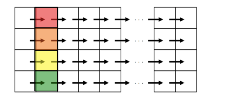
    for (int j =1; j < n; j++)
    #pragma omp parallel for
        for (int i = 0; i < m; i++)
            a[i][j] = 2 * a[i][j-1];
并行结果如下,数组每一列数据交给线程组进行并行化,一个线程一次得到的任务只有数组中一个元素,频繁的进行划分可能导致并行开销增大
- Loop exchange 后并行
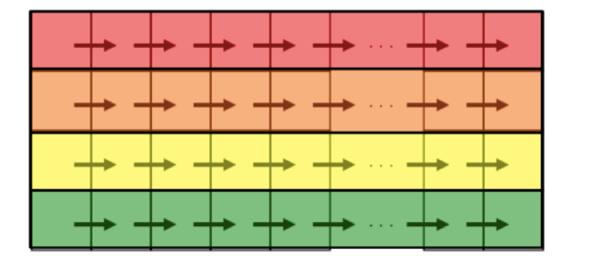
    #pragma omp parallel for
    for (int i =1; i < n; i++)
        for (int j= 0; j < m; j++)
            a[i][j] = 2 * a[i][j-1];
并行结果如下,直接将整个数组按行划分给线程,一个线程一次得到的任务有一行的,并行循环粒度较高
-
- Loop fission
- Expose a parallelizable loop
第八讲:MPI 编程模型,内容要点
1. 什么是 MPI 编程模型?
每个独立的处理器(processor)都有独立私有的内存,通过互联网络连接起来的分布式内存系统,利用消息传递来编程的模型。
2. 消息传递性并行编程模型的主要原则是什么?
1. The logical view of a machine supporting the message passing paradigm consists of p processes, each with its own exclusive address space
支持消息传递模型的系统的逻辑由 p 个处理器组成,每个处理器都有自己专用的地址空间
2. CONSTRAINTS(限制)
- Each data element must belong to one of the partitions of the space; hence, data must be explicitly partitioned and placed
每个数据元素必须属于某一个处理器的内存空间;因此,必须显式分区和放置数据。 - All interactions (read-only or read/write) require cooperation of two processes the process that has the data and the process that wants to access the data
拥有数据的进程和想要访问数据的进程的所有交互(只读或读/写)都需要两个进程的协作
3. These two constraints, while onerous (繁重), make underlying costs very explicit to the programmer
这两个约束虽然很繁重,但却使底层成本对程序员非常明确。
4. Message-passing programs are often written using the asynchronous or loosely synchronous paradigms
消息传递程序通常使用异步或松散同步的范例编写。
- In the asynchronous paradigm, all concurrent tasks execute asynchronously\
在异步模式中,所有并发任务都是异步执行的。
- In the loosely synchronous model, tasks or subsets of tasks synchronize to perform interactions. Between these interactions, tasks execute completely asynchronously\
在松散同步模型中,任务或任务子集同步以执行交互。在这些交互之间,任务完全异步执行
5. Most message-passing programs are written using the single program multiple data (SPMD) model
大多数消息传递程序是使用单程序多数据(SPMD)模型编写的。
3. MPI 中的几种 Send 和 Receive 操作包括原理和应用场景。
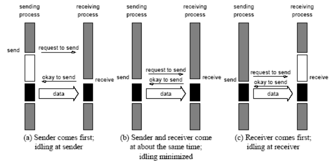
1. Non-buffered blocking
- A simple method for forcing (强制)send/receive semantics is for the
send operation to return only when it is safe to do so
强制 send/recv 语句的一个简单方法是 send 操作仅在安全时返回 - In the non-buffered blocking send, the operation does not return until
the matching receive has been encountered at the receiving process
在非缓冲阻塞 send 中,知道在传输过程中遇上匹配的 recv,操作返回 - Idling and deadlocks are major issues with nonbuffered blocking sends
空等、死锁问题存在
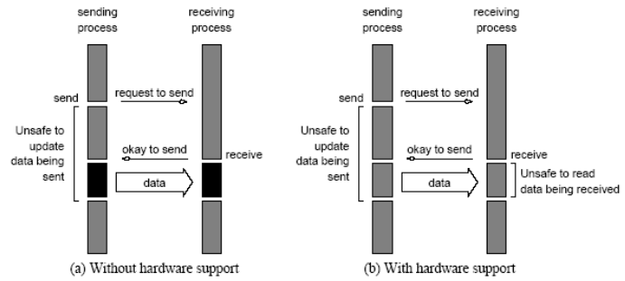
2. Buffered blocking
Non-buffered blocking => Buffered blocking
- In buffered blocking sends, the sender simply copies the data into the
designated buffer and returns after the copy operation has been completed. The data is copied at a buffer at the receiving end as well.
在缓冲块发送中,发送方只需将数据复制到指定的缓冲区中,并在复制操作完成后返回。数据也被复制到接收端的缓冲区中。 - Buffering alleviates idling at the expense of copying overheads
缓冲减少了空转的开销,而增加了复制开销。
Buffered blocking 的操作
- In buffered blocking sends, the sender simply copies the data into the
designated buffer and returns after the copy operation has been
completed.
在缓冲块 send 中,发送方只需要把数据复制到指定缓冲区中,并在复制操作完成后返回 - The data is copied at a buffer at the receiving end as well
也在接收端的缓冲区复制数据 - Buffering trades off idling overhead for buffer copying overhead
在空闲时缓冲区交换数据已抵消通信数据传输的开销
注意:\
a、缓冲区大小可能对性能影响显著
b、由于接受操作块(send-recv)的存在,使用缓冲块仍然可能出现死锁
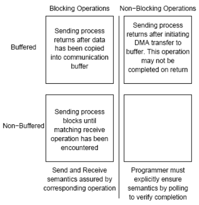
3. Non-blocking (非阻塞)
- The programmer must ensure semantics of the send and receive.
程序员必须确保发送和接收的语义正确。 - This class of non-blocking protocols returns from the send or receive operation before it is semantically safe to do so.
这类非阻塞协议在语义上安全之前从发送或接收操作返回。 - Non-blocking operations are generally accompanied by a check-status operation.
非阻塞操作通常伴随检查状态操作。 - When used correctly, these primitives are capable of overlapping communication overheads with useful computations.
如果使用正确,这些原语的通信开销可以与计算开销重叠起来 - Message passing libraries typically provide both blocking and non-blocking
primitives.
消息传递库通常同时提供阻塞原语和非阻塞原语。
4. MPI 的 send
- MPI_Send(标准模式)有缓存使用缓存,无缓存显式等待
- Will not return until you can use the send buffer (Non-local)
不会返回,直到可以使用缓存
- Will not return until you can use the send buffer (Non-local)
- MPI_Bsend(缓冲模式)
- Returns immediately and you can use the send buffer
立即返回和可以使用发送缓冲 - Related: MPI_buffer_attach(), MPI_buffer_detach()
- Returns immediately and you can use the send buffer
- MPI_Ssend(同步模式)需要多次握手
- Will not return until matching receive posted
不会返回,直到匹配上 recv - Send + synchronous communication semantics
发送+同步通信语义
- Will not return until matching receive posted
- MPI_Rsend(就绪模式)减少通信信息
- May be used ONLY if matching receive already ready
当且仅当匹配的 recv 已经准备好了则可以使用 - The sender provides additional information to the system that can save some overhead
发送者提供了额外的信息系统,可以节省部分开销
- May be used ONLY if matching receive already ready
- MPI_Isend(非阻塞标准模式)
- Nonblocking send, but you can NOT reuse the send buffer immediately
不能立即重用 send 缓冲区 - Related: MPI_Wait(), MPI_Test()
- Nonblocking send, but you can NOT reuse the send buffer immediately
- MPI_Ibsend
- MPI_Issend
- MPI_Irsend
5. Sending and Receiving Messages
- int MPI_Send(void *buf, int count, MPI_Datatype datatype, int dest, int tag, MPI_Comm comm) int MPI_Recv(void *buf, int count, MPI_Datatype datatype, int source, int tag, MPI_Comm comm, MPI_Status *status)
- MPI allows specification of wildcard arguments for both source and tag.
MPI 允许为源和标记指定通配符参数。 - If source is set to MPI_ANY_SOURCE , then any process of the communication domain can be the source of the message.
如果 source 设置为 MPI_ANY_SOURCE,则通信域的任何进程都可以是消息的源。 - If tag is set to MPI_ANY_TAG , then messages with any tag are accepted.
如果标记设置为 MPI_ANY_TAG 标记,则接受带有任何标记的消息。 - On the receive side, the message must be of length equal to or less than the length field specified.
在接收端,消息的长度必须等于或小于指定的长度字段。 - On the receiving end, the status variable can be used to get information
about the MPI_Recv operation.
在接收端,状态变量可用于获取有关 MPI_recv 操作的信息。 - The corresponding data structure contains:\
相应的数据结构包含
1
2
3
4
typedef struct MPI_Status {\
int MPI_SOURCE;\
int MPI_TAG;\
int MPI_ERROR; };
- The MPI_Get_count function returns the precise count of data items received
函数返回接收到的数据项的精确计数。
1
int MPI_Get_count(MPI_Status *status, MPI_Datatype datatype, int *count)
4. MPI 中的关键编程接口
- MPI_Init(int*argc,char***argv):函数,初始化
- MPI_Finalize():函数,结束时释放资源
- MPI_Comm_size:变量,定义 processes 的个数
- MPI_Comm_rank:变量,定义当前进程的序号
- MPI_Send():函数
- MPI_Recv():函数
- 一般以「MPI_」为前缀
- 相关进程形成进程组
1
2
3
4
5
MPI_Group_incl():进程集形成一个进程组\
MPI_Comm_create():为新的进程组创建一个通信子\
MPI_Comm_rank():为新的进程组定义序号\
MPI_Comm_free():释放进程组的资源\
MPI_Group_free():解进程组
5. 什么是通信子?
- A communicator defines a communication domain - a set of processes that are allowed to communicate with each other
通信子定义了一个通信域-允许彼此通信的一组进程。 - Information about communication domains is stored in variables of type
MPI_Comm
有关通信域的信息存储在 MPI_Comm 类型的变量中 - Communicators are used as arguments to all message transfer MPI routines
通信子被用作所有消息传输 MPI 例程的参数。 - A process can belong to many different (possibly overlapping) communication domains
一个进程可以属于许多不同的(可能重叠的)通信域 - MPI defines a default communicator called MPI_COMM_WORLD which includes all the processes
MPI 定义了一个名为 MPI_COMM_WORLD 的默认通讯子,其中包括所有进程
6. MPI 中解决死锁的方式有哪些
- Using non-blocking operations remove most deadlocks.
使用非阻塞操作可以避免大多数死锁 - In order to overlap communication with computation, MPI provides a pair of functions for performing non-blocking send and receive operations.
为了与计算重叠通信,MPI 提供了一对执行非阻塞发送和接收操作的函数MPI_Isend() 和 MPI_Irecv()
- 可以打断循环等待以避免死锁
- 同时 send 和 recv:MPI_Sendrecv();
7. MPI 中的集群通信操作子有哪些?原理是什么?
-
MPI provides an extensive set of functions for performing common collective communication operations.
MPI 提供了一套广泛的函数来执行公共的集体通信操作 -
Each of these operations is defined over a group corresponding to the communicator.
这些操作都是在通信子对应的一个进程组上定义的 -
All processors in a communicator must call these operations.
在同一个通信子中的处理器必须调用这些操作 -
The barrier synchronization operation is performed in MPI using:
1
int MPI_Barrier(MPI_Comm comm) (阻塞到所有进程完成调用)
The one-to-all broadcast operation is:
1
2
3
4
5
int MPI_Bcast(void *buf, int count, MPI_Datatype datatype,
int source, MPI_Comm comm) The all-to-one reduction operation is:
int MPI_Reduce(void *sendbuf, void *recvbuf, int count,
MPI_Datatype datatype, MPI_Op op, int target,
MPI_Comm comm)
- The all-to-one reduction operation is:
1
2
3
int MPI_Reduce(void *sendbuf, void *recvbuf, int count,
MPI_Datatype datatype, MPI_Op op, int target,
MPI_Comm comm)
-
Collective Commumication Operations
- If the result of the reduction operation is needed by all processes, MPI provides:
1
2
3
  >>>int MPI_Allreduce(void *sendbuf, void *recvbuf,
  >>>int count, MPI_Datatype datatype, MPI_Op op, MPI_Comm
comm)
-
To compute prefix-sums, MPI provides:
int MPI_Scan(void *sendbuf, void *recvbuf, int count, MPI_Datatype datatype, MPI_Op op, MPI_Comm comm)
-
The gather operation is performed in MPI using:
int MPI_Gather(void *sendbuf, int sendcount, MPI_Datatype senddatatype, void *recvbuf, int recvcount, MPI_Datatype recvdatatype, int target, MPI_Comm comm)
-
MPI also provides the MPI_Allgather function in which the data are gathered at all the processes.
int MPI_Allgather(void *sendbuf, int sendcount, MPI_Datatype senddatatype, void *recvbuf, int recvcount, MPI_Datatype recvdatatype,MPI_Comm comm)
- The corresponding scatter operation is:
int MPI_Scatter(void *sendbuf, int sendcount, MPI_Datatype senddatatype, void *recvbuf, int recvcount, MPI_Datatype recvdatatype, int source, MPI_Comm comm)
8 - MPI 编程模型
* 可参考文件 MPI.md
-
什么是 MPI 编程模型
MPI - the Message Passing Interface
* 参考老师 PPT,加粗部分即为重点内容。
MPI 是一个跨语言(编程语言如 C, Fortran 等)的通讯协议,用于编写并行计算机。支持点对点和广播。MPI 是一个信息传递应用程序接口,包括协议和和语义说明,他们指明其如何在各种实现中发挥其特性。MPI 的目标是高性能,大规模性,和可移植性。MPI 在今天仍为高性能计算的主要模型。与 OpenMP 并行程序不同,MPI 是一种基于信息传递的并行编程技术。消息传递接口是一种编程接口标准,而不是一种具体的编程语言。简而言之,MPI 标准定义了一组具有可移植性的编程接口。
-
消息传递并行编程模型的主要原则
* CH-8 p6
- 支持消息传递并行编程模型的设备,运行的多个进程应有自己独立的地址空间。
- 限制
- 每个数据单元必须归属于某一片划分好的地址空间,因此,必须显式划分并分配(place)数据。
- 无论是只读操作还是读写操作,都需要两个进程进行配合:拥有数据的进程以及操作发起的进程。
- 消息传递程序常常是异步或者松弛同步(loosely synchronous)的。
- 松弛同步:任务之间的交互同步进行,此外各个任务异步进行。
- 绝大多数的消息传递程序是由
single program multiple data - SPMD(单程序多数据流) 模型写的。
-
MPI 中的几种 Send 和 Receive 操作,包括原理和应用场景。
* CH-8 p9
Send 和 Receive 操作可分为以下三大类:
-
Non-buffered blocking 无缓冲阻塞
为保证传输安全,需要实现类似于「握手」的操作才能开始发送数据,容易导致空转和死锁。
-
Buffered blocking 缓冲阻塞
为了减轻空转和死锁现象,引入缓冲区。
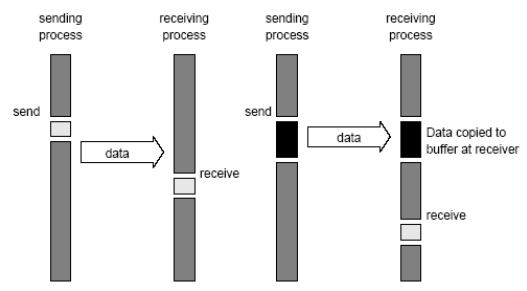
有通信硬件支持下:发送端不会中断接收方。
无通信硬件支持下:发送端中断接收方,将数据存入接收端缓冲区。
-
Non-blocking 非阻塞
-
非阻塞的协议是不安全的。
-
通常,非阻塞协议需要与状态检查操作(check-status operation)同步使用。
参见
MPI_Get_count(), MPI_Status1 2 3 4 5 6 7
typedef struct MPI_Status { int MPI_SOURCE; int MPI_TAG; int MPI_ERROR; }; int MPI_Get_count(MPI_Status *status, MPI_Datatype datatype, int *count)
-
若使用得当,非阻塞的原语能够将通信与有效计算重叠进行。(When used correctly, these primitives are capable of overlapping communication overheads with useful computations.)
-
总体比较:
-
-
MPI 中的关键编程接口
参见
MPI.md - $2 MPI基本函数 -
什么是通信子
参见
MPI.md - $4 MPI集群通信 - $4.0 组 & 通信子 -
MPI 中解决死锁的方式有哪些?
- 重排代码,避免死锁。
- 在发送时,添加接收缓冲区。
- 将自己(发送端)的地址空间作为发送缓冲区。
- 使用非阻塞的 send/receive 方法。
-
MPI 中的集群(群组)通信操作子有哪些?原理是什么?
MPI 定义了一系列扩展函数以实现集群通信操作,这些操作都是基于一个与通信子关联的群组定义的。通信子中的所有处理器必须调用这些操作。
参见
MPI.md - $4 MPI集群通信
9 - MPI 与 OpenMP 联合编程(*)
-
如何利用 MPI 实现 Matrix-Vector 乘积
对算式 $Ab=c$,有:
-
串行算法
略
-
三种并行算法
-
Row-wise block striped
- 将$A$各行拆分,$b$不动,各个进程完成两个向量的內积得到$c_i$.
- 调用
MPI_Allgatherv(...)聚合计算结果。 MPI_Allgatherv(...)参见MPI.md - $4 MPI集群通信 - $4.3 多对多通信
-
Column-wise block striped
-
将$A,b$各列拆分,各个进程按图示工作。
-
调用
MPI_Alltoall(...)传送计算结果。其中每个进程完成计算后得到上图中$c_{0j},c_{1j},c_{2j},c_{3j},c_{4j}$。最后分组加和。 -
MPI_Alltoall(...)参见MPI.md - $4 MPI集群通信 - $4.3 多对多通信
-
-
Checkerboard block
-
将$A$棋盘化分块,按照行划分同样对 b 进行分段。
-
需要注意,进程数 p 是否为完全平方数影响 b 分块的过程。
-
使用
MPI_Dims_create(...)以及MPI_Cart_create(...)新建拓扑关系通信子。 -
MPI_Dims_create(...),MPI_Cart_create(...)参见MPI.md - $5 MPI 逻辑分划 -
规约计算。
-
-
-
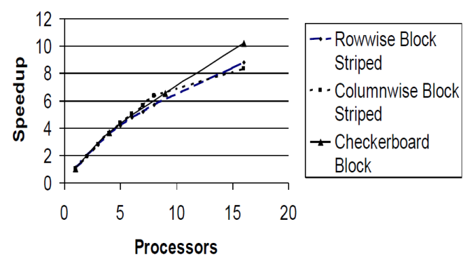
三种算法的性能比较
-
-
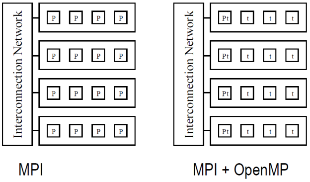
MPI 和 OpenMP 结合的优势是什么?
-
运行较只使用 MPI 快。
- 只使用 MPI 时,消息在m*k 个进程间传递;
- 联合编程时,消息在m 个含有 k 个线程的进程间传递,代价较低。
-
特别地,考虑不同处理器数量的情况:
-
2,4CPUs:MPI + OpenMP 较慢
MPI + OpenMP 是共享内存带宽(memory bandwidth)的,MPI-only 不是。
-
6,8CPUs:MPI + OpenMP 较快
更低的通信开销。
-
-
程序的更多部分可以并行实现。
只使用 MPI 时,不涉及消息传递的并行过程无法实现。
-
允许更多通信与有效计算的叠加(overlap)。
-
-
如何利用 MPI+OpenMP 实现高斯消元法
* CH - 9 p53
0 - 简介
-
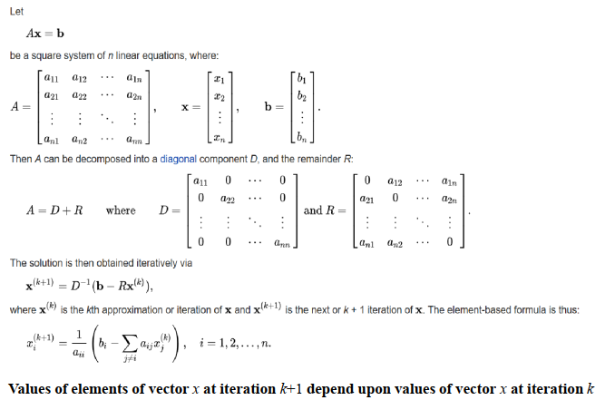
高斯消元法(Gaussian Elimination )
- 用于求解系数矩阵$A$是稠密(dense)矩阵的方程$Ax=b$
- 化简得到三角矩阵系统$Tx=c$,$T$为三角矩阵
- 回代求解$x$
-
稀疏矩阵系统(sparse system)
- 高斯消元法对稀疏系统的适应性不好。
- 高斯消元法使得稀疏矩阵新添很多非 0 元素
- 增加了存储需求
- 增加了操作次数
-
迭代方法(Iterative Methods)
- 存储需求较高斯消元法更小。
- 含有 0 元素的计算会被忽略,大大减少了计算量。
-
雅各比方法(Jacobi Method)
-
收敛性(Convergence)
- 一般只能达到较慢的收敛速度,很难实际应用。
1 - 新方案思想
- 对 MPI 进行概要分析(?Profile execution of MPI program)。
- 致力于在计算密集型的函数或代码段处加入 OpenMP 指令。
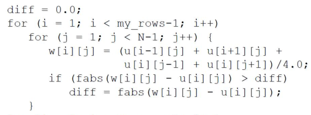
2 - 串行代码
-
find_steady_state()
-
无法并行执行最外层 for 循环的原因
for循环并不是规范形式(canonical form)- 包含
break语句 - 包含 MPI 功能函数
- 迭代之间存在数据依赖。
-
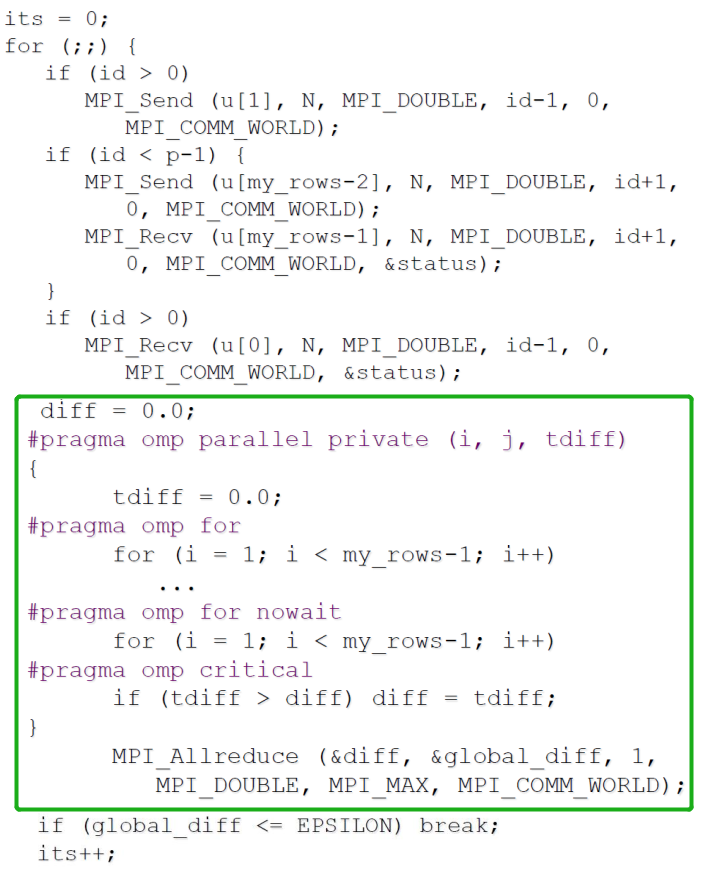
并行化本段 for 循环
- 处理
diff的更新(upadte)与检测(test)- 若考虑将
if语句置入临界区(critical section),会增加额外开销并且降低加速比。(Putting if statement in a critical section would increase overhead and lower speedup.) - 考虑引入私有变量
tdiff
- 若考虑将
- 在进行
MPI_Allreduce()规约之前,检测tdiff代替之前检测diff的步骤。
- 处理
3 - 并行化代码
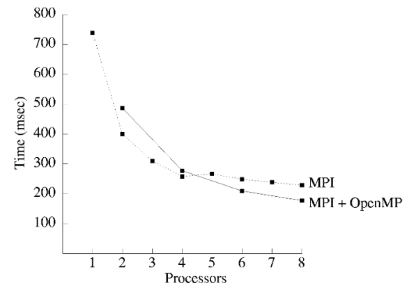
4 - 基准化测试
考虑以下环境:
系统:包含 4 个双核处理器节点的商业集群。
- C+MPI 在 1,2, … ,8 进程上运行
- C+MPI+OpenMP 在 1,2,3,4 进程上运行
- 每个进程包含 2 个线程
- 包含 2,4,6,8 线程
结果示意:
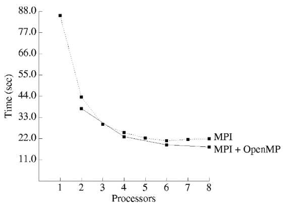
总结分析:
-
Hybrid C+MPI+OpenMP program uniformly faster than C+MPI program.
混合编程在速度上显著快于 MPI 编程。
-
Computation/communication ratio of hybrid program is superior.
混合编程的「计算通信比」更胜一筹。理解为单位通信次数/时间内有效计算量更大。
-
Number of mesh points per element communicated is twice as high per node for the hybrid program.
混合编程内每个通信元素的网格点数是程序节点数的两倍。
-
Lower communication overhead leads to 19% better speedup on 8 CPU.
混合编程在 8CPU 下通过减少通信开销实现了 19%的加速。
-
第九讲:MPI 与 OpenMP 联合编程,内容要点
1. 如何利用 MPI 实现 Matrix-vector 乘积?不同实现的特点是什么?
假设运算为 A*b=c,其中 A 为矩阵,b、c 为向量
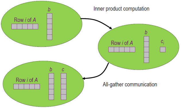
1. Rowwise Block Striped Matrix —— 行分块条形矩阵
-
Partitioning through domain decomposition
通过域分解划分 -
Primitive task associated with
原始任务关联- Row of matrix
矩阵的行 - Entire vector
整个向量
- Row of matrix
- 此时为 A 的第 i 行乘以 b 得到 c[i],在 All-gather communication 得到结果
-
有时会出现每个进程的结果个数不一样,所以不能使用 MPI_gather(因为要求每个进程的传输个数一样),所以使用 MPI_Allgatherv。
- Agglomeration and Mapping 合并与映射
- Static number of tasks
任务数量为静态划分 - Regular communication pattern (all-gather)
规则化通信 - Computation time per task is constant
每个任务的执行时间为常量 - Strategy:
- Agglomerate groups of rows
多行合并为一个子任务 —— 减少通信 - Create one task per MPI process
为每个 MPI 进程创建一个任务,分配子任务
- Agglomerate groups of rows
- Static number of tasks
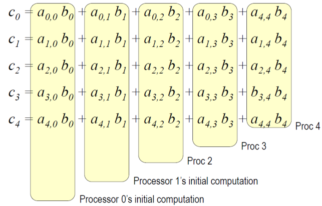
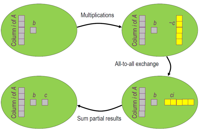
2. Columnwise Block Striped Matrix —— 列分块条形矩阵
-
Partitioning through domain decomposition
通过域分解进行划分 - Task associated with
原始任务关联- Column of matrix
矩阵的列 - Vector element
矢量元素
- Column of matrix
-
此时为 A 的第 i 列乘以 b[i]。
一般的做法为行列转置,即把结果部分 c[i]由不连续存储的列元素变成连续存储的行形式表示,再统计获得最终结果。图在 PPT 的 16 页。 - Agglomeration and Mapping
- Static number of tasks
任务数固定 - Regular communication pattern (all-to-all)
规则化通信 - Computation time per task is constant
计算时间恒定 - Strategy:
- Agglomerate groups of columns
把部分列元素作为一个子任务 - Create one task per MPI process
为每个 MPI 进程创建一个任务,分配子任务
- Agglomerate groups of columns
- Static number of tasks
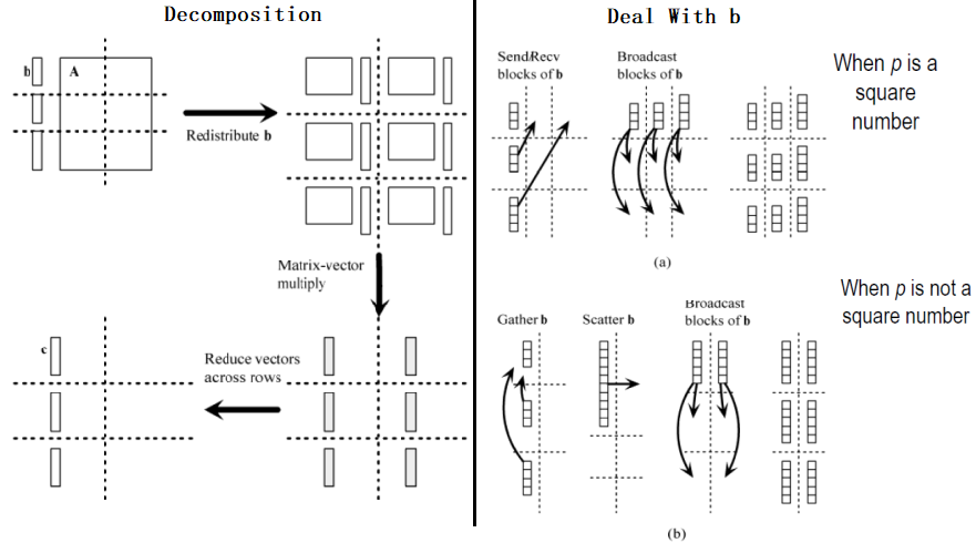
3. Checkerboard Block Decomposition —— 块划分
- Associate primitive task with each element of the matrix A
将原始任务与矩阵 A 的每个元素关联起来 - Each primitive task performs one multiply
每个基本任务执行一次乘法 - Agglomerate primitive tasks into rectangular blocks
将原始任务聚合成矩形块 - Processes form a 2-D grid
流程形成二维网格 -
Vector b distributed by blocks among processes in first column of grid
矢量 B 在网格第一列的进程之间按块分布 -
注意 PPT 中第 20 页和第 21 页的图。
- Redistributing Vector b
再分配向量 b- Step 1: Move b from processes in first row to processes in first column
步骤 1:将 B 从第一行的流程移到第一列的流程 - If p square
如果矩阵 A 的行数=列数 - First column/first row processes send/receive portions of b
直接第 i 部分的向量 b 对应矩阵的第一行的第 i 部分 - If p not square
如果矩阵 A 的行数!=列数 - Gather b on process 0, 0
先把 b 聚合到 process[0,0]的位置 - Process 0, 0 broadcasts to first row procs
再把 b 尽量平均地分配到第一行的各个部分 - Step 2: First row processes scatter b within columns
步骤 2:把第一行映射到其他行
- Step 1: Move b from processes in first row to processes in first column
2. MPI 和 OpenMP 结合的优势是什么?
MPI + OpenMP 可以执行的更快
- Lower communication overhead
更低的通讯开销- Message passing with mk processes, versus
- Message passing with m processes with k threads each
- More portions of program may be practical to parallelize
更多的部分可以并行 - May allow more overlap of communications with computations
通讯开销与计算开销重合的部分更多 - Hybrid Light-Weight Threads & Heavier-Weight Processes
混合了轻量级线程和重量级进程
3. 如何利用 MPI+OpenMP 实现高斯消元?
-
Sparse Systems
稀疏系统- Gaussian elimination not well-suited for sparse systems
高斯消元发并不适用与稀疏系统 - Coefficient matrix gradually fills with nonzero elements
系数矩阵逐渐填充非零元素- Increases storage requirements
增加存储要求 - Increases total operation count
增加总操作数
- Increases storage requirements
- Gaussian elimination not well-suited for sparse systems
-
Iterative Methods
迭代法- Iterative method: algorithm that generates a series of approximations to solution’s value
迭代法:生成一系列近似解值的算法 - Require less storage than direct methods
需要的存储量比直接方法少 - Since they avoid computations on zero elements, they can save a lot of computations
由于它们避免了零元素的计算,因此可以节省大量的计算。
- Iterative method: algorithm that generates a series of approximations to solution’s value
-
Methodology
方法- Profile execution of MPI program
MPI 执行配置操作的指令 - Focus on adding OpenMP directives to most compute-intensive function
专注于将 OpenMP 指令添加到大多数计算密集型功能中
- Profile execution of MPI program
第十讲:GPGPU、CUDA 和 OpenCL 编程模型,内容要点
- The CUDA Programming Model provides a general approach to organizing Data Parallel programs for heterogeneous, hierarchical platforms
- Currently, the only production-quality implementation is CUDA for C/C++ on Nvidia’s GPUs
- But CUDA notions of “Scalar Threads”, “Warps”, “Blocks”, and “Grids” can be mapped to other platforms as well
- A simple “Homogenous SPMD” approach to CUDA programming is useful, especially in early stages of implementation and debugging
-
But achieving high efficiency requires careful consideration of the mapping from computations to processors, data to memories, and data access patterns
- CUDA 编程模型提供了一种为异构、分层平台组织数据并行程序的通用方法。
- 目前,唯一的产品质量实现是在 NVIDIA 的 GPU 上实现用于 C/C++的 CUDA。
- 但 CUDA 的「标量线程」、「扭曲」、「块」和「网格」等概念也可以映射到其他平台。
- 对于 CUDA 编程,一种简单的「同质 SPMD」方法是有用的,特别是在实施和调试的早期阶段。
- 但是要实现高效率,需要仔细考虑从计算到处理器、从数据到存储器和数据访问模式的映射。
CUDA 的含义是什么
CUDA: Compute Unified Device Architecture
CUDA:计算统一设备架构
CUDA 的设计目标是什么,与传统的多线程设计有什么不同
Provide an inherently scalable environment for Data-Parallel programming across a wide range of processors (Nvidia only makes GPUs, however)
为跨多种处理器的数据并行编程提供内在可扩展的环境(不过,NVIDIA 只制造 GPU)。
Make SIMD hardware accessible to general-purpose programmers. Otherwise, large fractions of the available execution hardware are wasted!
使 SIMD 硬件对通用程序员可访问。否则,大部分可用的执行硬件都会被浪费掉!
PPT 上没找到很多与传统多线程设计的区别,但我觉得其实就很类似 SIMD 和 MIMD 的区别?(hhh)
- GPU programs (kernels) written using the Single Program Multiple Data (SPMD) programming model
- SPMD executes multiple instances of the same program independently, where each program works on a different portion of the data
- For data-parallel scientific and engineering applications, combining SPMD with loop strip mining is a very common parallel programming technique
- Message Passing Interface (MPI) is used to run SPMD on a distributed cluster
- POSIX threads (pthreads) are used to run SPMD on a shared memory system
- Kernels run SPMD within a GPU
- In the vector addition example, each chunk of data could be executed as an independent thread
- On modern CPUs, the overhead of creating threads is so high that the chunks need to be large
- In practice, usually a few threads (about as many as the number of CPU cores) and each is given a large amount of work to do
-
For GPU programming, there is low overhead for thread creation, so we can create one thread per loop iteration
- 使用单程序多数据(SPMD)编程模型编写的 GPU 程序(内核)。
- SPMD 独立执行同一程序的多个实例,其中每个程序处理数据的不同部分。
- 对于数据并行的科学和工程应用,将 SPMD 与循环条带挖掘相结合是一种非常常见的并行编程技术。
- 消息传递接口(MPI)用于在分布式集群上运行 SPMD。
- POSIX 线程(p 线程)用于在共享内存系统上运行 SPMD。
- 内核在 GPU 中运行 SPMD
- 在向量相加的示例中,每个数据块都可以作为一个独立的线程执行。
- 在现代 CPU 上,创建线程的开销是如此之高,以至于块需要很大。
- 在实践中,通常有几个线程(大约相当于 CPU 核心的数量),每个线程都有大量的工作要做。
- 对于 GPU 编程,线程创建的开销较低,因此我们可以在每次循环迭代中创建一个线程。
Scalability(扩展性)
- Cuda expresses many independent blocks of computation that can be run in any order;
- Much of the inherent scalability of the Cuda Programming model stems from batched execution of “Thread Blocks「;
-
Between GPUs of the same generation, many programs achieve linear speedup on GPUs with more 「Cores」; (线性加速比)
- CUDA 表示许多独立的计算模块,可以按任何顺序运行;
- CUDA 编程模型的许多固有可伸缩性源于「线程块」的成批执行;
- 在同一代图形处理器之间,许多程序在具有更多「核心」的图形处理器上实现线性加速;(线性加速比)
SIMD Programming
- Hardware architects love SIMD, since it permits a very space and energy-efficient implementation
- However, standard SIMD instructions on CPUs are inflexible, and difficult to use, difficult for a compiler to target
-
The Cuda Thread abstraction will provide programmability at the cost of additional hardware
- 硬件架构师喜欢 SIMD,因为它支持非常节省空间和节能的实施。
- 然而,CPU 上的标准 SIMD 指令是不灵活的,很难使用,编译器很难找到目标。
- CUDA 线程抽象将以额外硬件为代价提供可编程性
什么是 CUDA kernel
我个人的理解就是运行在设备上的 SPMD 核函数。
一个 kernel 结构如下:Kernel<<<Dg, Db, Ns, S>>>(param1, param2, ...)
- Dg:grid 的尺寸,说明一个 grid 含有多少个 block,为 dim3 类型,一个 grid 最多含有 655356553565535 个 block,Dg.x,Dg.y,Dg.z 最大值为 65535;
- Db:block 的尺寸,说明一个 block 含有多上个 thread,为 dim3 类型,一个 block 最多含有 1024(cuda2.x 版本)个 threads,Db.x 和 Db.y 最大值为 1024,Db.z 最大值 64;
(举个例子,一个 block 的尺寸可以是:
1024*1*1 | 256*2*2 | 1*1024*1 | 2*8*64 | 4*4*64等) - Ns:可选参数,如果 kernel 中由动态分配内存的 shared memory,需要在此指定大小,以字节为单位;
- S:可选参数,表示该 kernel 处在哪个流当中。
CUDA 的编程样例
自己补充:CUDA 的操作概括来说包含 5 个步骤:
- CPU 在 GPU 上分配内存:cudaMalloc;
- CPU 把数据发送到 GPU:cudaMemcpy;
- CPU 在 GPU 上启动内核(kernel),它是自己写的一段程序,在每个线程上运行;
- CPU 把数据从 GPU 取回:cudaMemcpy;
- CPU 释放 GPU 上的内存:cudaFree。
其中关键是第 3 步,能否写出合适的 kernel,决定了能否正确解决问题和能否高效的解决问题。
CUDA 的线程分层结构
Cuda 对线程做了合适的规划,引入了 grid 和 block 的概念,block 由线程组成,grid 由 block 组成,一般说 blocksize 指一个 block 放了多少 thread;gridsize 指一个 grid 放了多少个 block。
Parallelism in the Cuda Programming Model is expressed as a 4-level Hierarchy
- A Stream is a list of Grid sthat execute in-order. Fermi GPUs execute multiple Streams in parallel
- A Grid is a set of up to 232 thread Blocks executing the same kernel
- A Thread Block is a set of up to 1024 [512 pre-Fermi] Cuda Threads
- Each Cuda Thread is an independent, lightweight, scalar execution context
- Groups of 32 threads form Warps that execute in lockstep SIMD
Cuda 编程模型中的并行性被表示为一个 4 层的层次结构。
- 流(Stream)是按顺序执行的 Grid 列表。Fermi GPU 并行执行多个流。
- 网格(Grid)是一组最多 232 个执行同一内核的线程块。
- 线程块是一组最多 1024(512 预费米)Cuda 线程。
- 每个 cuda 线程都是一个独立的、轻量级的标量执行上下文。
- 32 个线程组成的组形成在 lockStepSIMD 中执行的扭曲。
CUDA Thread
- Logically, each CUDA Thread : – Has its own control flow and PC, register file, call stack, … – Can access any GPU global memory address at any time – Identifiable uniquely within a grid by the five integers: threadIdx.{x,y,z}, blockIdx.{x,y}
-
Very fine granularity: do not expect any single thread to do a substantial fraction of an expensive computation – At full occupancy, each Thread has 21 32‐bit registers – … 1,536 Threads share a 64 KB L1 Cache / shared mem – GPU has no operand bypassing networks: functional unit latencies must be hidden by multithreading or ILP (e.g. from loop unrolling)
- 逻辑上,每个 CUDA 线程:
- 有自己的控制流程和 PC,注册文件,调用堆栈,.。
- 可以随时访问任何 GPU 全局内存地址。
- 可通过以下五个整数在网格中唯一标识:线程标识。{x,y,z},块标识。{x,y}。
- 非常精细的粒度:不要指望任何一个线程都能完成昂贵的计算中的很大一部分。
- 在完全占用时,每个线程有 21 个 32 位寄存器。
- .1,536 个线程共享 64 KB L1 缓存/_SHARED_mem。
- GPU 没有操作数绕过网络:功能单元延迟必须通过多线程或 ILP 隐藏(例如,从循环展开)
CUDA Warp
- The Logical SIMD Execution width of the CUDA processor
- A group of 32 CUDA Threads that execute simultaneously – Execution hardware is most efficiently utilized when all threads in a warp execute instructions from the same PC. – If threads in a warp diverge (execute different PCs), then some execution pipelines go unused (predication) – If threads in a warp access aligned, contiguous blocks of DRAM, the accesses are coalesced ( 合并 ) into a single high bandwidth access – Identifiable uniquely by dividing the Thread Index by 32
-
Technically, warp size could change in future architectures – But many existing programs would break
- CUDA 处理器的逻辑 SIMD 执行宽度。
- 一组同时执行的 32 个 CUDA 线程。
- 当扭曲中的所有线程从同一台 PC 执行指令时,执行硬件的使用效率最高。
- 如果扭曲中的线程发散(执行不同的 PC),则某些执行管道将未使用(预测)。
- 如果扭曲访问中的线程对齐了 DRAM 的连续块,则将访问合并(合并)为单个高带宽访问。
- 通过将线程索引除以 32 来唯一标识。
- 从技术上讲,Warp 的大小在未来的体系结构中可能会发生变化
- 但许多现有的程序将会中断。
Cuda Thread Block
- A Thread Block is a virtualized multi-threaded core
- Number of scalar threads, registers, and __shared memory are configured dynamically at kernel-call time
- Consists of a number (1-1024) of Cuda Threads, who all share the integer identifiers blocladx. {x, y}
- …executing a data parallel task of moderate granularity
- The cacheable working-set should fit into the 128 KB (64 KB, pre-Fermi) Register File and the 64 KB (16 KB) Li
- Non-cacheable working set limited by GPU DRAM capacity
- All threads in a block share a (small) instruction cache
-
Threads within a block synchronize via barrier-intrinsics and communicate via fast, on-chip shared memory
- 线程块是虚拟化的多线程内核。
- 在内核调用时动态配置标量线程、寄存器和_共享内存的数量。
- 由 CudaThread 的一个数字(1-1024)组成,这些线程共享整数标识符 blocladx。{x,y}。
- …。执行中等粒度的数据并行任务。
- 可缓存工作集应适合 128KB(64KB,Pre-Fermi)注册表文件和 64KB(16KB)LI。
- 受 GPU DRAM 容量限制的不可缓存工作集。
- 块中的所有线程共享(小型)指令缓存。
- 块中的线程通过屏障-内部同步,并通过快速的片上共享内存进行通信
Cuda Grid
- A set of Thread Blocks performing related computations
- All threads in a single kernel call have the same entry point and function arguments, initially differing only in blockIdx. {x,y}
- Thread blocks in a grid may execute any code they want, e.g. switch (blockIdx.x) incurs no extra penalty
- Performance portability/scalability requires many blocks per grid: 1-8 blocks execute on each SM
-
Thread blocks of a kernel call must be parallel sub-tasks
- Program must be valid for any interleaving of block executions
- The flexibility of the memory system technically allows Thread Blocks to communicate and synchronize in arbitrary ways
- E.G. Shared Queue index: OK! Producer-Consumer: RISKY!
- 一组执行相关计算的线程块。
- 单个内核调用中的所有线程都具有相同的入口点和函数参数,最初仅在 block Idx 中有所不同。{x,y}。
- 网格中的线程块可以执行它们想要的任何代码,例如 Switch(block Idx.x)不会受到额外的惩罚。
- 性能、可移植性/可扩展性要求每个网格有多个数据块:在每个 SM 上执行 1-8 个数据块。
- 内核调用的线程块必须是并行子任务。
- 程序必须对块执行的任何交错有效。
- 内存系统的灵活性在技术上允许线程块以任意方式进行通信和同步。
- 共享队列索引:好的!生产者-消费者:风险!
Cuda Stream
- A sequence of commands (kernel calls, memory transfers) that execute in order.
- For multiple kernel calls or memory transfers to execute concurrently, the application must specify multiple streams. – Concurrent Kernel execution will only happen on Fermi and later – On pre‐Fermi devices, Memory transfers will execute concurrently with Kernels.
CUDA 的内存分层结构
- Each CUDA Thread has private access to a configurable number of registers – The 128 KB (64 KB) SM register file is partitioned among all resident threads – Registers, stack spill into (cached, on Fermi) 「local」 DRAM if necessary
- Each Thread Block has private access to a configurable amount of scratchpad memory – The Fermi SM’s 64 KB SRAM can be configured as 16 KB L1 cache + 48 KB scratchpad (暂存器), or vice‐versa* – Pre‐Fermi SM’s have 16 KB scratchpad only – The available scratchpad space is partitioned among resident thread blocks, providing another concurrency‐state tradeoff
- Thread blocks in all Grids share access to a large pool of 「Global」 memory, separate from the Host CPU’s memory. – Global memory holds the application’s persistent state, while the thread‐local and block‐local memories are temporary – Global memory is much more expensive than on‐chip memories: O(100)x latency, O(1/50)x (aggregate) bandwidth
- On Fermi, Global Memory is cached in a 768KB shared L2
- There are other read-only components of the Memory Hierarchy that exist due to the Graphics heritage of Cuda
- The 64 KB Cuda Constant Memory resides in the same DRAM as global memory, but is accessed via special read-only 8 KB per-SM caches
- The Cuda Texture Memory also resides in DRAM and is accessed via small per-SM read-only caches, but also includes interpolation hardware
- This hardware is crucial for graphics performance, but only occasionally is useful for general-purpose workloads
- The behaviors of these caches are highly optimized for their roles in graphics workloads ?
- Each CUDA device in the system has its own Global memory, separate from the Host CPU memory – Allocated via cudaMalloc()/cudaFree() and friends
- Host <-> Device memory transfers are via cudaMemcpy() over PCI‐E, and are extremely expensive – microsecond latency, ~GB/s bandwidth
-
Multiple Devices managed via multiple CPU threads
- 每个 CUDA 线程都可以私有地访问可配置的寄存器数量-128KB(64KB)SM 寄存器文件在所有驻留线程中进行分区-寄存器、堆栈溢出到(缓存的,在 Fermi 上)「本地」DRAM(如有必要)。
- 每个线程块都可以私有地访问可配置数量的暂存盘内存-费米 SM 的 64KB 内存可以配置为 16KB L1 缓存+48KB 暂存板(暂存器),反之亦然*-Pre-FermiSM 仅有 16KB 暂存板-可用暂存板空间在常驻线程块之间进行分区,从而提供另一个并发状态权衡。
- 所有网格中的线程块共享对大型「全局」内存池的访问权限,这些内存池与主机 CPU 的内存分开。-全局内存保存应用程序的持久状态,而线程本地和块本地内存是临时的-全局内存比片上内存昂贵得多:O(100)x 延迟,O(1/50)x(聚合)带宽。
- 在 Fermi 上,全局内存缓存在 768KB 共享 L2 中。
- 由于 CUDA 的图形遗产,内存层次结构中存在其他只读组件。
- 64 KB cuda 常量内存与全局内存驻留在同一 DRAM 中,但通过特殊的只读 8 KB/SM 缓存进行访问。
- cuda 纹理内存也驻留在 dram 中,可以通过小的 per-sm 只读缓存进行访问,但也包括插值硬件。
- 此硬件对于图形性能至关重要,但仅偶尔对通用工作负载有用。
- 这些缓存的行为是否针对其在图形工作负载中的角色进行了高度优化?
- 系统中的每个 CUDA 设备都有自己的全局内存,独立于主机 CPU 内存-通过 cudaMalloc()/cudafree()和 Friend()分配。
- 主机<->设备内存传输是通过 cudaMemcpy()通过 PCI-E 进行的,并且是非常昂贵的-微秒延迟,~Gb/s 带宽。
- 通过多个 CPU 线程管理多个设备
CUDA 中的内存访问冲突
Using Per-Block Shared Memory
- Each SM has 64 KB of private memory, divided 16KB/48KB (or 48KB/16KB) into so hardware‐managed scratchpad and hardware‐managed, non‐coherent cache – Pre‐Fermi, the SM memory is only 16 KB, and is usable only as so hardware‐managed scratchpad
-
Unless data will be shared between Threads in a block, it should reside in registers - On Fermi, the 128 KB Register file is twice as large, and accessible at higher bandwidth and lower latency
- Pre‐Fermi, register file is 64 KB and equally fast as scratchpad
- 每个 SM 都有 64 KB 的私有内存,将 16KB/48KB(或 48KB/16KB)分为由硬件管理的暂存板和由硬件管理的非一致性缓存。
- 在费米之前,SM 内存只有 16KB,只能作为硬件管理的暂存盘使用。
- 除非数据将在块中的线程之间共享,否则它应该驻留在寄存器中
- 在 Fermi 上,128KB 的寄存器文件是原来的两倍,并且可以在更高的带宽和更低的延迟下访问。
- preFermi,注册文件为 64KB,速度与便签簿一样快
Atomic Memory Operations
cuda 提供了原生的原子操作,例如
-
CUDA provides a set of instructions which execute atomically with respect to each other
- Allow non‐read‐only access to variables shared between threads in shared or global memory
- Substantially more expensive than standard load/stores
- With voluntary consistency, can implement e.g., spin locks!
- CUDA 提供了一组相互独立执行的指令。
- 允许对共享内存或全局内存中的线程之间共享的变量进行非只读访问。
- 比标准货物/商店贵得多。
- 具有自愿性一致性,可实现例如旋转锁定!
Voluntary Memory Consistency
- By default, you cannot assume memory accesses are occur in the same order specified by the program
- Although a thread’s own accesses appear to that thread to occur in program order
- To enforce ordering, use memory fence instructions
- __threadfence_block(): make all previous memory accesses visible to all other threads within the thread block
- __threadfence(): make previous global memory accesses visible to all other threads on the device
-
Frequently must also use the volatile type qualifier
- Has same behavior as CPU C/C++: the compiler is forbidden from register‐promoting values in volatile memory
- Ensures that pointer dereferences produce load/store instructions
- Declared as volatile float *p; *p must produce a memory ref.
- 默认情况下,不能假定内存访问的顺序与程序指定的顺序相同。
- 虽然线程自己的访问似乎是按程序顺序进行的。
- 要执行排序,请使用内存围栏说明。
- _throfence_block():使所有先前的内存访问对该线程块中的所有其他线程都可见。
- _throfence():使以前的全局内存访问对设备上的所有其他线程可见。
- 还必须经常使用易失性类型限定符。
- 具有与 CPU C/C+相同的行为:禁止编译器在易失性内存中执行寄存器提升值。
- 确保指针取消引用生成加载/存储指令。
- 声明为易失性浮点p;p 必须生成内存引用。
OpenCL 运行时编译过程
Platform
- 查询并选择一个 platform
- 在 platform 上创建 context
- 在 context 上查询并选择一个或多个 device
Running time
- 加载 OpenCL 内核程序并创建一个 program 对象
- 为指定的 device 编译 program 中的 kernel
- 创建指定名字的 kernel 对象
- 为 kernel 创建内存对象
- 为 kernel 设置参数
- 在指定的 device 上创建 command queue
- 将要执行的 kernel 放入 command queue
- 将结果读回 host
资源回收
第十一讲:MapReduce 并行编程模型,内容要点
- MapReduce Programming Model
- Typical Problems Solved by MapReduce
- MapReduce Examples
- A Brief History
- MapReduce Execution Overview
- Hadoop
MapReduce
- A simple and powerful interface that enables automatic parallelization and distribution of large-scale computations, combined with an implementation of this interface that achieves high performance on large clusters of commodity PCs.」
-
More simply, MapReduce is A parallel programming model and associated implementation
- 一种简单而强大的接口,可实现大规模计算的自动并行化和分布,并可在大型商品 PC 集群上实现高性能。
- 更简单地说,MapReduce 是一种并行编程模型及其相关实现
Some MapReduceTerminology
- Job–A 「full program」 -an execution of a Mapper and Reducer across a data set
- Task –An execution of a Mapper or a Reducer on a slice of data
- a.k.a. Task-In-Progress (TIP)
- Task Attempt –A particular instance of an attempt to execute a task on a machine
一些 MapReduce 终端(猜测翻译成专有名词更合适?)。
- Job-「完整程序」-跨数据集执行映射器和还原器。
- 任务-在数据切片上执行映射器或还原器。
- 别名。正在进行的任务(TIP)。
- 任务尝试-尝试在计算机上执行任务的特定实例
为什么会产生 MapReduce 并行编程模型
- 全社会数据产生的速度非常快
- 大数据的呈现出指数增长速度
Motivation: Large Scale Data Processing
- Want to process lots of data ( >1TB)
- Want to parallelize across hundreds/thousands of CPUs
- … Want to make this easy
动机:大规模数据处理。
- 要处理大量数据(>1TB)。
- 希望跨数百/数千个 CPU 并行化。
- …。想让这件事变得简单
MapReduce 与其他并行编程模型如 MPI 等的主要区别是什么
MapReduce 的主要流程是什么
-
Process data using special map() and reduce() functions
- The map() function is called on every item in the input and emits a series of intermediate key/value pairs
- All values associated with a given key are grouped together
- The reduce() function is called on every unique key, and its value list, and emits a value that is added to the output
- The map() function is called on every item in the input and emits a series of intermediate key/value pairs
-
使用特殊 map()和 reduce()函数处理数据。
- 对输入中的每个项调用 map()函数,并发出一系列中间键/值对。
- 将与给定键关联的所有值组合在一起。
- 对每个唯一的键及其值列表调用 reduce()函数,并发出一个添加到输出中的值
- 对输入中的每个项调用 map()函数,并发出一系列中间键/值对。
Map
- Records from the data source (lines out of files, rows of a database, etc) are fed into the map function as key*value pairs: e.g., (filename, line)
-
map() produces one or more intermediate values along with an output key from the input
- 将来自数据源的记录(文件的行数、数据库的行数等)作为键*值对输入到 map 函数中:例如(文件名、行)。
- map()从输入生成一个或多个中间值以及输出键
Reduce
- After the map phase is over, all the intermediate values for a given output key are combined together into a list
-
reduce() combines those intermediate values into one or more final values for that same output key
- 映射阶段结束后,给定输出键的所有中间值将合并到一个列表中。
- Reduce()将这些中间值组合为同一输出键的一个或多个终值
MapReduce 的简单实现。如 Hello World 例子
使用 python 实现的分词程序。
map.py
1
2
3
4
5
6
7
8
9
10
11
12
13
14
15
import sys
import time
import re

p = re.compile(r'\w+')
for line in sys.stdin:
        ss = line.strip().split(' ')
        for s in ss:
        #time.sleep(1)
        if len(p.findall(s))<1:
            #print s
            continue
        s = p.findall(s)[0].lower()
            if s.strip() != "":
                print "%s\t%s" % (s, 1)
reduce.py
1
2
3
4
5
6
7
8
9
10
11
12
13
14
15
16
17
import sys

current_word = None
sum = 0

for line in sys.stdin:
    word, val = line.strip().split('\t')

    if current_word == None:
        current_word = word

    if current_word != word:
        print "%s\t%s" % (current_word, sum)
        current_word = word
        sum = 0
    sum += int(val)
print "%s\t%s" % (current_word, str(sum))
MapReduce 具有哪些容错措施
- Master detects worker failures
- Re-executes completed & in-progress map() tasks
- Re-executes in-progress reduce() tasks
-
Master notices particular input key/values cause crashes in map(), and skips those values on re-execution
- Effect: Can work around bugs in third-party libraries!
- Master 检测工人故障。
- 重新执行已完成和正在进行的 map()任务。
- 重新执行正在进行的 reduce()任务。
- Master 在 map()中注意到特定的输入键/值导致崩溃,并在重新执行时跳过这些值。
- 效果:可以解决第三方库中的错误!
MapReduce 存在哪些优化点
Optimizations
- No reduce can start until map is complete
- A single slow disk controller can rate-limit the whole process
- Master redundantly executes 「slow-moving」 map tasks; uses results of first copy to finish
- 「Combiner」 functions can run on same machine as a mapper
-
Causes a mini-reduce phase to occur before the real reduce phase, to save bandwidth
- 在 map 完成之前,不能开始 reduce。
- 单个慢速磁盘控制器可以对整个过程进行速率限制。
- Master 冗余地执行「缓慢移动」的 map 任务;使用第一次复制的结果来完成。
- 「组合器」函数可以像映射器一样在同一台计算机上运行。
- 导致在实际减少阶段之前出现一个小减少阶段,以节省带宽
MapReduce 可以解决的问题有哪些
Greatly reduces parallel programming complexity
- Reduces synchronization complexity
- Automatically partitions data
- Provides failure transparency
-
Handles load balancing
- 降低同步复杂性。
- 自动划分数据。
- 提供故障透明度。
- 处理负载平衡
Typical Problems Solved by MapReduce
- Read a lot of data
- Map: extract something you care about from each record
- Shuffle and Sort
- Reduce: aggregate, summarize, filter, or transform
- Write the results
-
Outline stays the same, but map and reduce change to fit the problem
- 阅读大量数据。
- Map:从每条记录中提取您关心的内容。
- 洗牌和排序。
- 减少:聚合、汇总、筛选或转换。
- 写下结果。
- 大纲保持不变,但映射并减少更改以适应问题
第十二讲:基于 Spark 的分布式计算,内容要点
Spark 与 Hadoop 的区别和联系
它扩展了广泛使用的 MapReduce 计算模型。高效的支撑更多计算模式,包括交互式查询和流处理。spark 的一个主要特点是能够在内存中进行计算,及时依赖磁盘进行复杂的运算,Spark 依然比 MapReduce 更加高效。
传统 MapReduce 的主要缺点是什么
MapReduce is great at one-pass computation, but inefficient for multi-pass algorithms. No efficient primitives for data sharing
- State between steps goes to distributed file system
- Slow due to replication & disk storage
MapReduce 在单程计算方面很好,但对于多路算法效率较低。没有有效的数据共享原语。
- 步骤之间的状态转到分布式文件系统。
- 由于复制和磁盘存储而速度较慢
Spark 中的 RDD 如何理解
- RDD 是 Spark 的核心数据模型,但是个抽象类,全称为 Resillient Distributed Dataset,即弹性分布式数据集。
- RDD 在抽象上来说是一种元素集合,包含了数据。它是被分区的,分为多个分区,每个分区分布在集群中的不同节点上,从而让 RDD 中的数据可以被并行操作。(分布式数据集)
- RDD 通常通过 Hadoop 上的文件,即 HDFS 文件或者 Hive 表,来进行创建;有时也可以通过应用程序中的集合来创建。
- RDD 最重要的特性就是,提供了容错性,可以自动从节点失败中恢复过来。即如果某个节点上的 RDDpartition,因为节点故障,导致数据丢了,那么 RDD 会自动通过自己的数据来源重新计算该 partition。这一切对使用者是透明的。
- RDD 的数据默认情况下存放在内存中的,但是在内存资源不足时,Spark 会自动将 RDD 数据写入磁盘。(弹性)
Spark 样例程序
In this example, we use a few transformations to build a dataset of (String, Int) pairs called counts and then save it to a file.
1
2
3
4
5
text_file = sc.textFile("hdfs://...")
counts = text_file.flatMap(lambda line: line.split(" ")) \
             .map(lambda word: (word, 1)) \
             .reduceByKey(lambda a, b: a + b)
counts.saveAsTextFile("hdfs://...")
第十三讲:离散搜索与负载均衡
1. 深度优先搜索的主要流程
从图中某顶点 v 出发: (1)访问顶点 v; (2)依次从 v 的未被访问的邻接点出发,对图进行深度优先遍历;直至图中和 v 有路径相通的顶点都被访问; (3)若此时图中尚有顶点未被访问,则从一个未被访问的顶点出发,重新进行深度优先遍历,直到图中所有顶点均被访问过为止。(百度)
- 开始遍历当前节点的子树
- 如果一个节点的所有子树都被遍历过, 则回溯
时间复杂度$\theta(b^k)$, 空间复杂度$\theta(k)$, b 为宽度, k 为深度
2. 深度优先搜索的复杂度
假设状态空间树中的平均分支因子(每个节点的子节点数(平均值))为 b,搜索一棵深度为 k 的树需要检索:
个结点。空间复杂度为 Θ(k)
3. 并行深度优先搜索的主要设计思想
每个处理器处理一个子树
- Send nodes near the bottom of the stack(发送堆栈底部附近的结点),适用于均匀搜索空间;分配成本低。
- Send nodes near the cutoff depth(发送截止深度附近的结点),使用强启发式(尝试分配搜索空间中可能包含解决方案的部分)可以获得更好的性能。
- Send half the nodes between the bottom and the cutoff depth(发送底部和截止深度之间的一半结点),适用于均匀不规则的搜索空间。
4. 动态负载均衡的三种方法,以及每种方法的额外开销复杂度
均衡负载
- Asynchronous round robin(ARR),异步循环,每个进程维护一个计数器并以循环方式发出请求。
- Global round robin(GRR),全局循环,系统维护一个全局计数器,并以循环方式在全局发出请求。
- Random polling(RP),随机轮询,请求随机选择的工作流程。
额外开销复杂度
我们将 v(p)定义为每个处理器在收到至少一个工作请求之后的工作请求总数;假设任意点的最大工作量是 W;则工作请求总数为 O(V(p)logW)。
- ARR:V(p) = O(p²)在最坏情况下
- GRR:V(p) = p
- RP:
最坏情况下 V(p)是无穷的。 平均状况下 V(p) = O(plogp)
- ARR:W = O(p²logp)
- GRR:最坏情况下 W = O(p²logp)
- RP:W = O(plog²p)
- ARR 性能较差,因为它会发出大量的工作请求。
- GRR 调度由于计数器上的争用而性能较差,尽管它发出的请求数最少。
- RP 是一个理想的折衷办法。
5. 最优搜索的处理过程
6. 并行最优搜索的主要思想的实现方式
7. 什么是加速比异常,主要份哪几类
- 由于处理器探索的搜索空间是在运行时动态确定的,实际工作可能会有很大的差异。
- 使用 P 处理器产生大于 P 的加速的执行被称为加速异常。使用 P 处理器的小于 P 的加速被称为减速异常。
- 加速异常也表现在最佳优先搜索算法中。
- 如果启发式函数是好的,那么并行的 best-first 搜索中所做的工作通常比串行搜索中所做的工作要多。
性能优化综合
负载均衡
- 负载均衡主要有哪些方式?分别有什么特点?
- 静态、动态负载均衡适用的场景是什么?
- 如何选择任务的粒度?
理想情况下, 所有处理器在程序运行时同时计算, 并同时结束他们被分派的任务.
问题: 实现更好的负载均衡
- 需要所有处理器充分执行
- 需要低开销的负载均衡管理实现
- 减小调度开销
- 减小同步开销
静态分派与动态分派
- 他们是共存的选择
- 使用前置的负载均衡知识取减少负载不均衡和任务管理同步开销
方式
静态分派(Static assignment)
静态负载均衡
在每个线程运行前, 每个线程被分派的任务规模已经被确定. 即预先分派每个线程执行的任务. 这可以在编译期间分派, 也可以在运行期间依据运行参数分派(比如数据大小, 线程数量).
特点
- 优点
- 简单
- 零运行时开销
- 缺点
适用场景
任务的开销(执行时间)和任务的数量是可预测的
半静态分派(「Semi-static」 assignment)
周期性地进行预测并再动态分派, 在相邻再分配的时间间隔内, 为静态分派
适用场景
任务的开销在较近的未来是可预测的.
动态分派(Dynamic assignment)
程序在运行时动态地分派任务.
适用场景
任务的开销和数量是不可预测的
动态负载均衡的优化
任务的粒度
考虑用工作队列的方式实现动态分派. 一个共享的工作队列, 里面有一些待完成的任务.
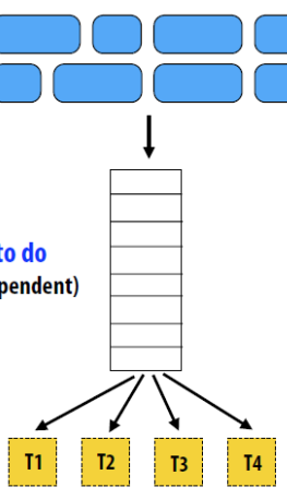
worker thread 可以执行两种操作
- 从队列中弹出一个任务
- 从队列中推入新的任务
我们来分析一下任务的粒度对这种动态负载均衡方式的影响
粒度小
- 大量的小任务, 使得动态负载均衡效果好
- 高分派开销
粒度大
- 负载均衡效果差
- 分派次数少, 开销小
如何选择任务的粒度
- 大量的小粒度任务保证了良好的动态负载均衡效果
- 大粒度任务减少了分派管理的开销
理想的粒度还取决于许多因素.
长尾现象(long pole)
考虑下列任务
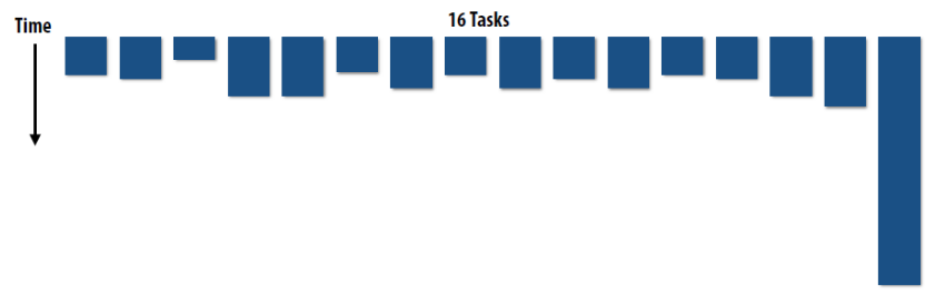
如果简单地进行分派, 可能造成负责不均衡
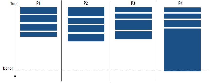
解决的办法
- 将任务划分为大量的小人物
- 可能将大任务切分为小任务, 使得负载更均衡
- 增加同步开销
- 可能没效果(如果长任务是连续的)
- 先分派大任务执行
- 执行大任务的线程相比其他线程可能执行的任务的数量更少.
- 需要能预测任务的开销
使用分布式队列减少同步开销
这样可以避免所有 workers 需要进行同时同步.
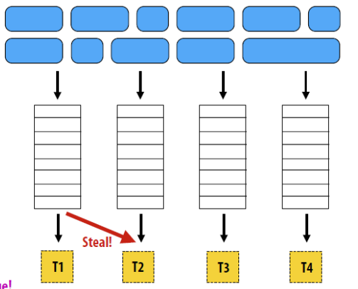
当 worker 线程队列为空时, 会从别的队列中偷(steal)任务
特点
- 仅当 steal 的时候有通信和同步的开销
- 增加了局部性, 每个线程基本只运行本地创建的任务
问题
- Who to steal from?
- How much to steal?
- How to detect program termination?
- Ensuring local queue access is fast
任务依赖
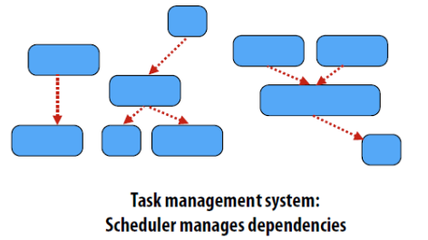
- 队列中的任务仅当所有的依赖任务都完成时才能被弹出队列, 分派给 worker
减少通信开销
- Latency 和 Throughput 的定义
- 通信时间的计算方法
- 并行程序中通信产生的原因
- 什么是天然通信?什么是人为通信?举例
- 什么是运算密度?
- 人为通信包括哪些?
- 减少通信代价的方式有哪些?
减少通信代价方法
- Reduce overhead of communication to sender/receiver
- Send fewer messages, make messages larger (amortize overhead)
- Coalesce (合并)many small messages into large ones
- Reduce delay
- Application writer: restructure code to exploit locality
- HW implementor: improve communication architecture
- Reduce contention
- Replicate contended resources (e.g., local copies, fine-grained locks)
- Stagger access to contended resources
- Increase communication/computation overlap
- Application writer: use asynchronous communication (e.g., async messages)
- HW implementor: pipelining, multi-threading, pre-fetching, out-of-order exec
- Requires additional concurrency in application (more concurrency than number of execution units)
优化通信
- Inherent vs. artifactual communication
- Inherent communication is fundamental given how the problem is decomposed and how work is assigned
- Artifactual communication depends on machine implementation details (often as important to performance as inherent communication)
- Improving program performance
- Identify and exploit locality: communicate less (increase arithmetic intensity)
- Reduce overhead (fewer, large messages)
- Reduce contention
- Maximize overlap of communication and processing (hide latency so as to not incur cost)
阻塞型 send/recieve

- send: 在确保接收方接收到数据才返回
- recv: 将数据拷贝到本地缓存才返回
阻塞型 send/recv 如何避免死锁
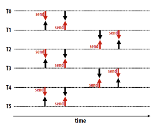
非阻塞型 send/recv
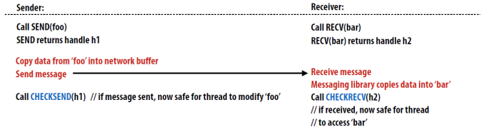
- send: 立马返回, 需要保证发送缓冲区之后一段时间不改变
- recv: 立马返回, 需要使用 checksend(), checkrecv()检查状态
Latency 与 Throughput
传输延迟(Latency): 一个操作完成需要的时间.
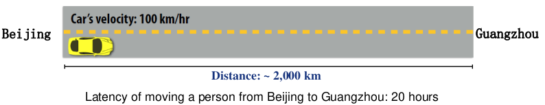
吞吐量(Throughput/Bandwidth): 操作执行时的速度
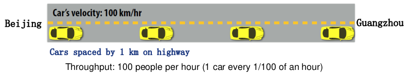
增加吞吐量的方法
-
加快传输速度
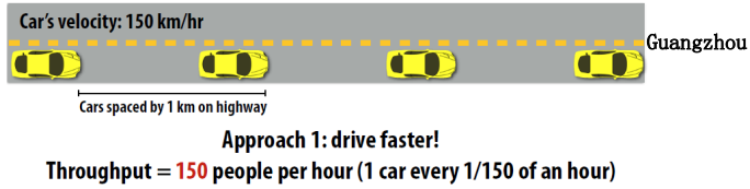
-
加大带宽
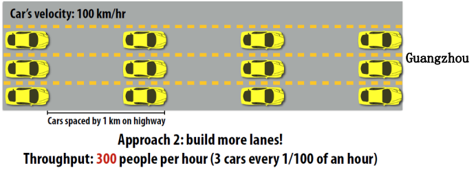
通信与 pipline
上一节的讨论让我们知道, 虽然不可用减少 latency, 但可以增加 pipline 程度来提高 throughput.
对于无 pipline 的通信而言, 开销如下
\[T(n)=T_0+\frac{n}{B}\]- $T_0$: latency
- n: 传输字节数
- $B$: bandwidth
对于以下情景考虑 pipline 方式
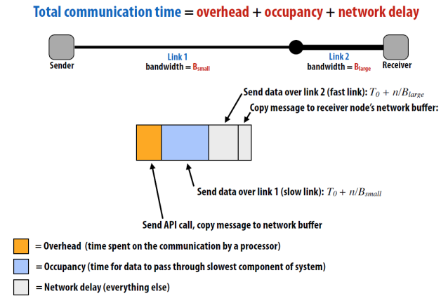
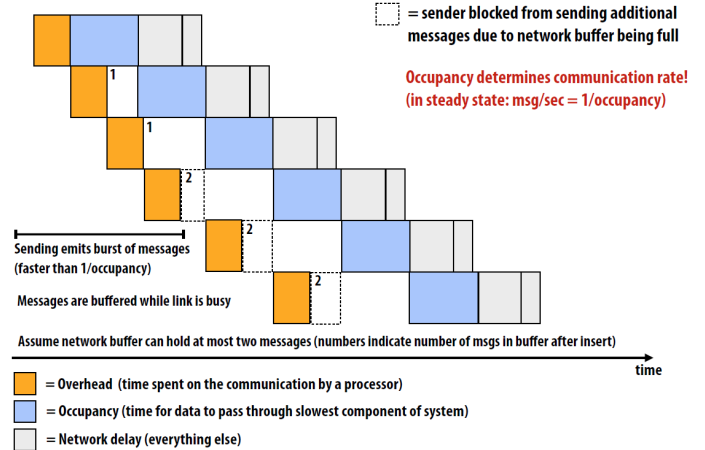
通信开销
通信时间=本地开销+传输开销+传播开销+异地开销
通信开销=通信时间-overlap 部分
运算密度(Arithmetic intensity)
运算密度: 运算数量/通信数量
通信产生的原因
天然通信(Inherent communication)
并行算法中必须要的通信, 是算法的组成部分
information that fundamentally must be moved between processors to carry out the algorithm given the specified assignment (assumes unlimited capacity caches, minimum granularity transfers, etc.)
如何减少? 通过改进算法
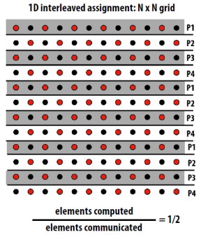
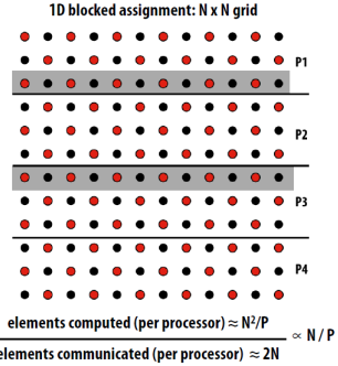
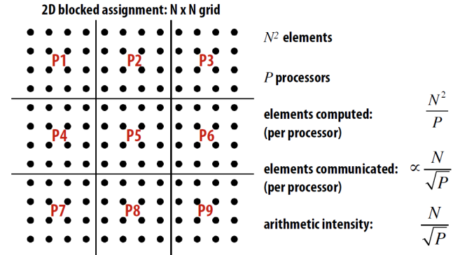
人为通信(artifactual communication)
all other communication (artifactual communication results from practical details of system implementation)
- System might have a minimum granularity of transfer (result: system must communicate more data than what is needed)
-
System might have rules of operation that result in unnecessary communication
- 受通信粒度影响
- Cache Size
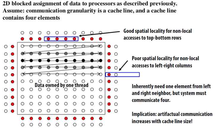
- 任务划分

- 改变布局
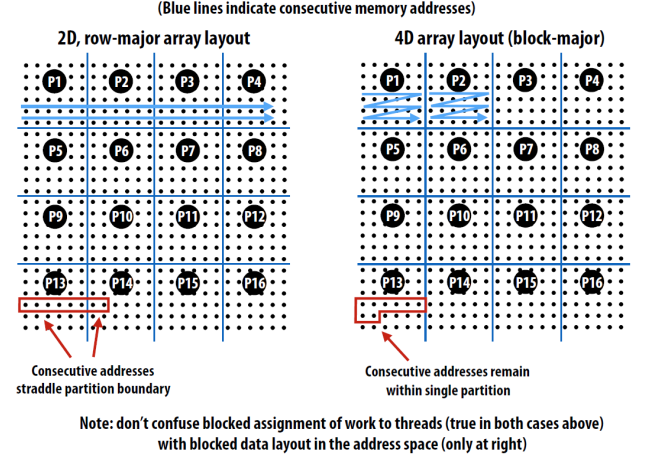
- Cache Size
增强局部性
- Cache 冲突包含哪些类型?
- 提高 Cache 局部性的方式有哪些?
Cache 冲突类型
- Cold miss: First time data touched. Unavoidable in a sequential program
- Capacity miss: Working set is larger than cache. Can be avoided/reduced by increasing cache size.
- Conflict miss: Miss induced by cache management policy.Can be avoided/reduced by changing cache associativity, or data access pattern in application.
- Communication miss (new): Due to inherent or artifactual communication in parallel system
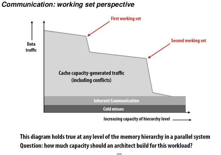
减少 Cache Miss
改变访问顺序
考虑 row-major traversal 的访问方法

其中蓝色为在 Cache 中的部分, 所以我们需要 change grid traversal order
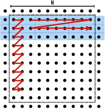
融合循环
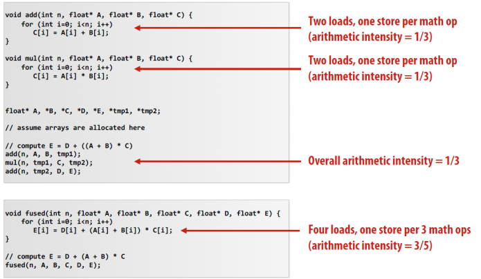
本地处理器共享数据
- Exploit sharing: co-locate tasks that operate on the same data
- Schedule threads working on the same data structure at the same time on the same processor
- Reduces inherent communication
减少数据竞争
- 减少数据竞争的方式有哪些?
Contention occurs when many requests to a resource are made within a small window of time
解决方法
parallelize over cells
One possible answer is to decompose work by cells: for each cell, independently compute particles within it (eliminates contention because no synchronization is required)
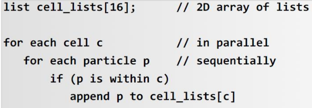
parallelize over particles
assign one particle to each CUDA thread. Thread computes cell containing particle, then atomically updates list.
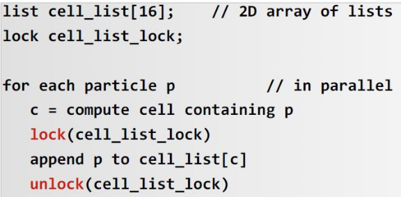
use finer-granularity locks
Alleviate contention for single global lock by using per-cell locks
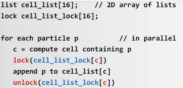
compute partial results + merge
- Example: create M thread blocks (at least as many thread blocks as SMX cores)
- Each block assigned N/M particles
- All threads in thread block update same grid
- Enables faster synchronization: contention reduced by factor of M and also cost of synchronization is lower because it is performed on block-local variables (in CUDA shared memory)
- Requires extra work: merging the M grids at the end of the computation
- Requires extra memory footprint: Store M grids of lists, rather than 1
第十四讲:性能优化之一,内容要点
1. 负载均衡主要有哪些方式?分别有什么他特点?
- 静态分配:
- 预先决定分配的工作线程,不一定在编译时确定(分配算法可能取决于运行时参数,如输入数据大小、线程数等)。(分配包括按块和按行)
Assignment of work to threads is pre-determined,Not necessarily determined at compile-time (assignment algorithm may depend on runtime parameters such as input data size, number of threads, etc.) - 简单,本质上是零运行时开销
simple, essentially zero runtime overhead (in this example: extra work to implement assignment is a little bit of indexing math)
- 预先决定分配的工作线程,不一定在编译时确定(分配算法可能取决于运行时参数,如输入数据大小、线程数等)。(分配包括按块和按行)
- 「半静态「分配:(注:「半静态」分配属于静态分配的一种)
- 工作成本短时间可以预测
Cost of work is predictable for near-term future - 应用程序定期对自身进行配置并重新调整分配
Application periodically profiles itself and re-adjusts assignment
- 工作成本短时间可以预测
- 动态分配:
- 程序在运行时动态的确定分配,以确保负载分布良好(任意的执行时间和执行点数是不可预测的)
Program determines assignment dynamically at runtime to ensure a well distributed load. (The execution time of tasks, or the total number of tasks, is unpredictable.) - 使用工作队列动态分配
Dynamic assignment using a work queue
- 程序在运行时动态的确定分配,以确保负载分布良好(任意的执行时间和执行点数是不可预测的)
2. 静态、动态负载均衡适用的场景是什么?
- 静态
- 当工作的成本(执行时间)和工作量是可预测的(这样程序员就可以提前完成一项很好的任务)
When the cost (execution time) of work and the amount of work is predictable - 当工作是可预测的,但不是所有的工作都有相同的成本
When work is predictable, but not all jobs have same cost (see example below) - 当关于执行时间的统计数据是已知的(例如,平均成本相同)
When statistics about execution time are known (e.g., same cost on average)
- 当工作的成本(执行时间)和工作量是可预测的(这样程序员就可以提前完成一项很好的任务)
- 动态
不知道工作的成本与资源
3. 如何选择任务的粒度?
有用比处理器更多的任务(很多小任务可以通过动态分配好工作负载平衡)
Useful to have many more tasks* than processors (many small tasks enables good workload balance via dynamic assignment)
- 激发小粒度的任务:
Motivates small granularity tasks
但希望尽可能少的任务的开销最小化管理任务
But want as few tasks as possible to minimize overhead of managing the assignment- 激发大粒度任务
Motivates large granularity tasks
理想的粒度取决于许多因素(在这门课中共同的主题:必须知道你的工作量,和你的机器)
Ideal granularity depends on many factors (Common theme in this course: must know your workload, and your machine)
4. Cilk_spawn 的原理是什么?
- cilk_spawn foo (args);语义:调用 foo,但与标准函数调用不同,调用者可以继续异步执行 foo。
- 注意,cilk_spawn 抽象没有指定如何或何时计划执行派生调用。只是它们可以与调用者并发运行(以及由调用者生成的所有其他调用)
- cilk_spawn foo(args); Semantics: invoke foo, but unlike standard function call, caller may continue executing asynchronously with execution of foo.
- notice that the cilk_spawn abstraction does not specify how or when spawned calls are scheduled to execute. only that they may be run concurrently with caller(and with all other calls spawned by caller)
5. Cilk_sync 的原理是什么?
- 语义:当当前函数生成的所有调用都已完成时返回。(与派生调用「同步」) 注意:在包含 cilk_spawn 的每个函数的末尾都有一个隐式 cilk_sync(含义:当一个 Cilk 函数返回时,与该函数相关的所有工作都完成了)
- cilk_sync 确实是调度上的一个约束。所有派生调用必须在 cilk_sync 返回之前完成。
- Semantics: returns when all calls spawned by current function have completed. (「sync up」 with the spawned calls) Note: there is an implicit cilk_sync at the end of every function that contains a cilk_spawn (implication: when a Cilk function returns, all work associated with that function is complete)
- cilk_sync does serve as a constraint on scheduling. All spawned calls must complete before cilk_sync returns.
6. Cilk_spawn 的调度方式有哪些?各自有什么特点?
-
先运行延续
- 在执行任何迭代之前,调用方线程派生都可以用于所有迭代
- 如果没有窃取,执行顺序与删除 cilk_spawn 的程序非常不同。
- run continuation first(“child stealing”)
- caller thread spawns work for all iterations before executing any of it
- If no stealing,execution order is very different than that of program with cilk_spawn removed.
- 孩子优先
- 调用方线程只创建一个要窃取的项(表示所有剩余迭代的延续)
- 如果没有发生串列,线程将从工作队列中不断弹出 continuation,并为新的 continuation(更新值为 i)排队
- 执行顺序与删除派生的程序相同。
- run child first(“continuation stealing”)
- caller thread only creates one item to steal(continuation that represents all remaining iterations)
- If no straling occurs, thread continually pops continuation from work queue, enqueues new continuation(with updated value of i)
- Order of execution is the same as for program with spawn removed.
7. Cilk_spawn 中任务在不同线程之间 steal 的过程。
- 人均出列
- 工作队列实现为 dequeue(双端队列)
- 本地线程从「尾部」(底部)推送/弹出
- 远程线程从「头部」(顶部)窃取
- 存在高效的无锁 dequeue 实现
- 工作队列实现为 dequeue(双端队列)
-
dequeue per worker
- Work queue implemented as a dequeue (double ended queue)
- Local thread pushes/pops from the 「tail」 (bottom)
- Remote threads steal from 「head」 (top)
- Efficient lock-free dequeue implementations exist
- Work queue implemented as a dequeue (double ended queue)
- 随机选择受害人
- 空闲线程随机选择一个线程尝试从队列顶部窃取
- 从 dequeue 头中窃取……
- 减少与本地线程的争用:本地线程访问 dequeue 的部分与窃取线程不同!
- 偷工作开始调用树:这是一个「大」的作品,所以执行偷的成本摊销(分摊)再未来计算
- 最大化局部性:(结合 run-child-first 政策)本地线程作用于本地调用树的一部分
- random choice of victim
- Idle threads randomly choose a thread to attempt to steal from
- Stealing from top of dequeue…
- Reduces contention with local thread: local thread is not accessing same part of dequeue that stealing threads do! \
- Steals work at beginning of call tree: this is a 「larger」 piece of work, so the cost of performing a steal is amortized (分摊) over longer future computation
- Maximizes locality: (in conjunction with run-child-first policy) local thread works on local part of call tree
8. Cilk_sync 的几种实现方式。
- 不偷
如果线程没有窃取任何工作,那么在同步点上就不做任何事
-
no stealing
If no work has been stolen by threads, then there’s nothing to do at the sync point
- stalling join (具体请参考 ppt14 50-56 页,看图比较形象)
- 启动 fork 的线程必须预先形成同步
- 因此,它等待所有生成的工作完成。在本例中,线程 0 是引发 fork 的线程。
- stalling join
- Thread that initiates the fork must preform the sync
- Therefore it waits for all spawned work to be complete. In the case, thread 0 is the thread initating the fork.
- greedy policy(具体参考 57-62 页)
Click 框架简介
Reference
- Cilk_spawn 的原理是什么?
- Cilk_sync 的原理是什么?
- Cilk_spawn 的调度方式有哪些?各自有什么特点?
- Cilk_spawn 的任务在不同线程之间 steal 的过程
- Cilk_sync 的几种实现方式
Scheduling fork-join parallelism
常见的并行编程范式有两种
- 数据并行(Data parallelism), 比如 openmp 的 parallel for.
- 对每个执行单元创建新线程, 比如 pthread
Fork-join pattern: Natural way to express independent work in divide-and-conquer algorithms
Cilk 框架的几个重要函数
-
cilk_spawn foo(args): 「fork」 (create new logical thread of control)Semantics: invoke foo, but unlike standard function call, caller may continue executing asynchronously with execution of foo.
-
cilk_sync: 「join」 Semantics: returns when all calls spawned by current function have completed. Note: there is an implicit cilk_sync at the end of every function that contains
注意
- 上述的函数只是一种抽象,
cilk_spawn只保证 callee 可能与 caller 和其他 callees 一起执行 cilk_sync起到调度上的约束作用
例子
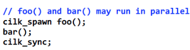
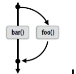
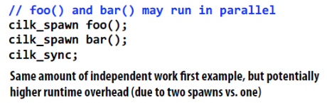
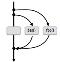
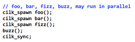
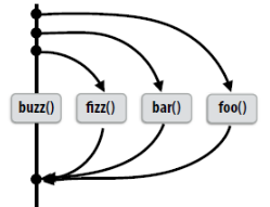
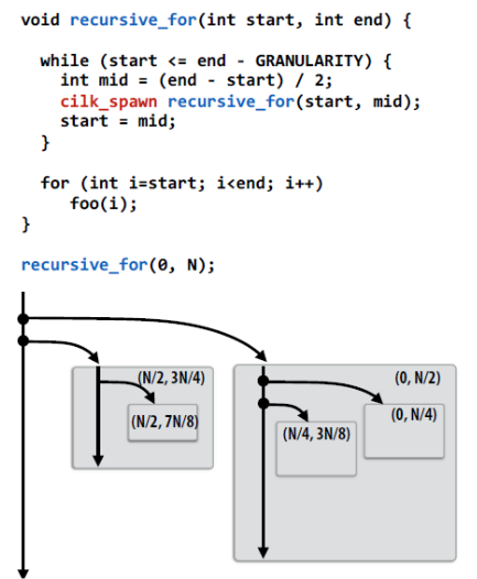
并行化快速排序
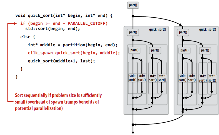
如何编写 fork-join 程序
- Main idea: expose independent work (potential parallelism) to the system using cilk_spawn
- Recall parallel programming rules of thumb
- Want at least as much work as parallel execution capability (e.g., program should probably spawn at least as much work as there are cores)
- Want more independent work than execution capability to allow for good workload balance of all the work onto the cores
- 「parallel slack」 = ratio of independent work to machine’s parallel execution capability (in practice: ~8 is a good ratio)
- But not too much independent work so that granularity of work is too small (too much slack incurs overhead of managing fine-grained work)
Cilk 的 fork-join 的调度
The Cilk Plus runtime maintains pool of worker threads
- all threads created at application launch
- as many worker threads as execution contexts in the machine
cilk_spawn将程序划分为两部分
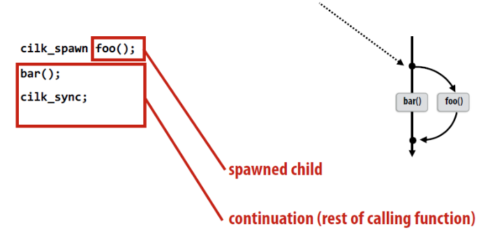
- spawned child
- continuation(rest of calling function)
以下是几个实现的细节
- 每个 thread 都有一个 work queue, 实现为 dequeue (double ended queue)
- Local thread pushes/pops from the 「tail」 (bottom)
- Remote threads steal from 「head」 (top)
- Efficient lock-free dequeue implementations exist
- thread
cilk_spawn后会将原 work 划分为spawned child和continuation, 选取一个执行, 另一个放到work queue - 闲置线程会从其他线程的 work queue 偷 work(Idle threads 「steal」 work from busy threads)
那么, 现在有个问题, 当一个线程cilk_spawn后, 它是先执行spawned child还是continuation
- continuation first: 先执行 continuation
- child first: 先执行 spawned child
以这个代码为例
1
2
3
4
for (int i = 0; i < N; i++) {
    cilk_spawn foo(i);
}
cilk_sync;
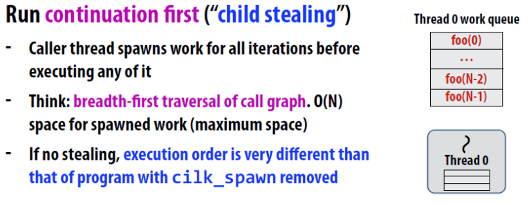
执行顺序为 0, 1, 2 …
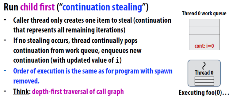
执行顺序为 N-1, N-2, N-3 …
work stealing 的实现
- Idle threads randomly choose a thread to attempt to steal from
- Stealing from top of dequeue…
- Reduces contention with local thread: local thread is not accessing same part of dequeue that stealing threads do!
- Steals work at beginning of call tree: this is a 「larger」 piece of work, so the cost of performing a steal is amortized (分摊) over longer future computation
- Maximizes locality: (in conjunction with run-child-first policy) local thread works on local part of call tree
sync 的实现
descriptor
-
如果没有 stealing, 其他线程无事可做, sync 的实现为
nop -
stalling join: Thread that initialtes the fork must perform the sync
对于每个由cilk_spawn和cilk_sync界定的代码块, 创建一个descriptor, 来描述这个代码块任务的完成情况
- id: 标识代码块
- spawn: work 数量
- done: 完成的 work 数量
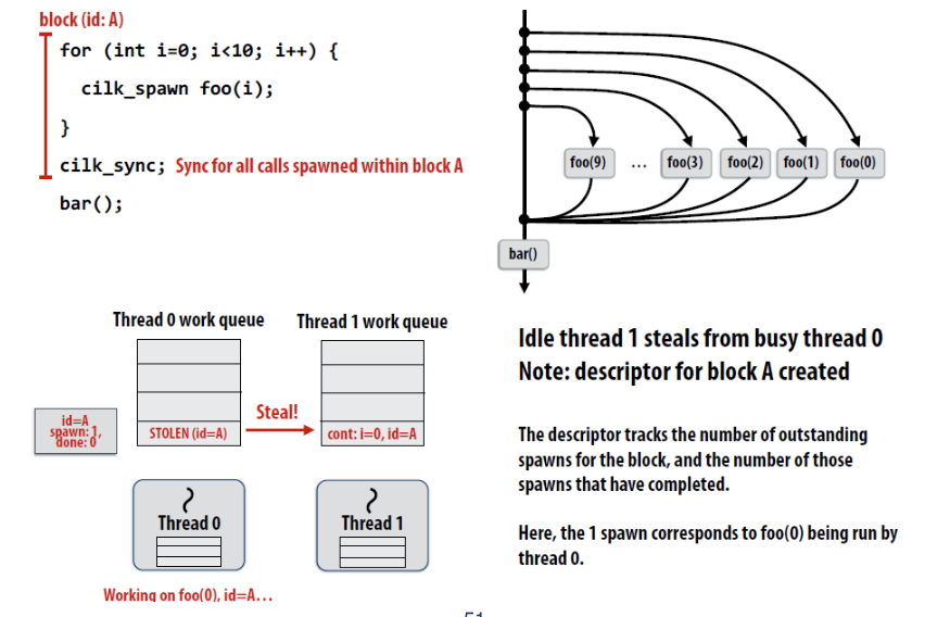
greedy policy
所有线程如果无事可做, 都会试图去偷任务. nitiated spawn thread 不一定是在 sync 后继续执行 work 的 initiated spawn thread
第十五讲:性能优化之二,内容要点
1. Latency 和 Throughput 的定义。
- 延迟:网络延迟是指各式各样的数据在网络介质中通过网络协议(如 TCP/IP)进行传输,如果信息量过大不加以限制,超额的网络流量就会导致设备反应缓慢,造成网络延迟
- 吞吐量:单位时间内成功地传送数据的数量
(以上来自百度百科)
2. 通信时间的计算方法。
通信时间 = 程序通信时间+占有时间+网络延迟\
- overhead:处理器用于通信的时间\
- occupancy: 数据通过系统最慢组件的时间\
- network delay: 其他的东西
Total communication time = overhead + occupancy + network delay\
- overhead: time spent on the communication by a processor\
- occupancy: time for data to pass through slowest component of system\
- network delay: everything else
3. 并行程序中通信产生的原因。
- 处理器与其缓存之间的通信
- 处理器与存储器之间的通信。(内存在同一台机器上)
- 处理器和远程存储器之间的通信。(集群中另一个节点上的内存,通过发送网络消息访问)
- communication between a processor and its cache
- conmmunication between processor and memory(e.g., memory on same machine)
- conmmunication between processor and a remote memory(e.g., memory on another node in the cluster, accessed by sending by sending a network message)
4. 什么是天然通信?什么是人为通信?举例说明。
天然通信:根据指定的分配(假设无限容量缓存、最小粒度传输等),必须在处理器之间移动才能执行算法的信息
Inherent communication: information that fundamentally must be moved between processors to carry out the algorithm given the specified assignment (assumes unlimited capacity caches, minimum granularity transfers, etc.)
- 行与行之间的通信是天然通信
人为通信:所有其他通信(人为沟通源于系统实现的实际细节)
Artifactual communication: all other communication (artifactual communication results from practical details of system implementation)
- 举例见 6 题
5. 什么是运算密度?
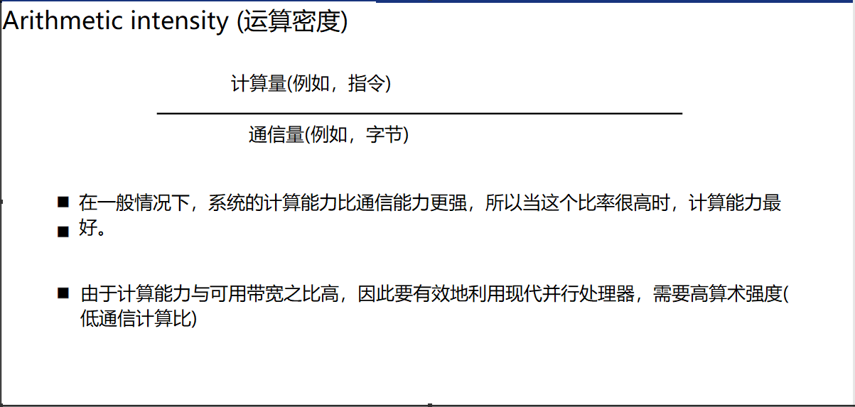
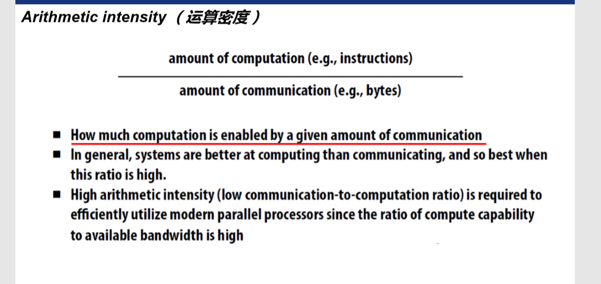
6. 人为通信包含哪些?
- 系统需要更小的粒度:所以系统需要更多的通信(程序加载一个 4 字节浮点值,但整个 64 字节高速缓存线必须是内存传输(比需要多 16 倍的通信)
System might have a minimum granularity of transfer (result: system must communicate more data than what is needed)
Program loads one 4-byte float value but entire 64-byte cache line must be transferred from memory (16x more communication than necessary)
- 系统可能有操作规则造成不必要的通信:(程序存储 16 个连续的 4 字节浮点值,但整个 64 字节高速缓存行,首先从内存加载,然后存储到内存(2x 开销)
System might have rules of operation that result in unnecessary communication: Program stores 16 consecutive 4-byte float values, but entire 64-byte cache line is first loaded from memory, and then subsequently stored to memory (2x overhead)
- 数据在分布式内存中的位置不佳(数据不驻留在访问数据最多的处理器附近)
Poor placement of data in distributed memories (data doesn’t reside near processor that accesses it the most)
- 有限的复制容量(由于本地存储(例如,缓存)太小,无法在访问之间保留相同的数据,因此多次与处理器通信)
Finite replication capacity (same data communicated to processor multiple times because local storage (e.g., cache) is too small to retain it between accesses)
7. Cache 冲突包含哪些种类?
- cold miss: 有限的复制容量(由于本地存储(例如缓存)太小,无法在访问之间保留相同的数据,因此多次与处理器通信)。在顺序程序中不可避免
Cold miss: First time data touched. Unavoidable in a sequential program - capacity miss: 工作集大于缓存。可以通过增加缓存大小来避免/减少。
Capacity miss: Working set is larger than cache. Can be avoided/reduced by increasing cache size. - conflict miss: 缓存管理策略导致的遗漏。可以通过改变应用程序中的缓存关联或数据访问模式来避免/减少。
Conflict miss: Miss induced by cache management policy. Can be avoided/reduced by changing cache associativity, or data access pattern in application. - communication miss: 由于并行系统中固有的或人为的通信
Communication miss : Due to inherent or artifactual communication in parallel system
8. 提高 Cache 局部性的方式有哪些?
- 通过改变网格遍历顺序来改进时间局部性
- 通过融合循环改进时间局部性
- 通过共享数据提高算法强度
- Improving temporal locality by changing grid traversal order
- Improving temporal locality by fusing loops
- Improve arithmetic intensity by sharing data
9. 减少数据竞争的方式有哪些?
- 分布式工作队列可以减少争用
- 在大型并行机器上创建粒子数据结构网格
- 粒子层次并行化
- 使用细粒度锁
- distributed work queues serve to reduce contention
- create grid of particles data structure on large parallel machine
- parallelize over particles
- use finer-granularity locks
10. 减少通信代价的方式有哪些?
- 减少发送方/接收方的通信开销
- 发送更少的消息,使消息更大(摊销开销)
- 合并(合)并成大的许多小消息
- 减少延迟
- 应用程序编写器:重构代码以利用局部性
- HW 实现者:改进通信架构
- 减少争用
- 复制竞争资源(例如,本地副本、细粒度锁)
- 错开对争用资源的访问
- 增加沟通/计算重叠
- 应用程序编写器:使用异步通信(例如,异步消息)
- HW 实现者:流水线,多线程,预取,无序执行
- 应用程序中需要额外的并发性(并发性多于执行单元的数量)
- Reduce overhead of communication to sender/receiver
- Send fewer messages, make messages larger (amortize overhead)
- Coalesce (合并)many small messages into large ones
- Reduce delay
- Application writer: restructure code to exploit locality
- HW implementor: improve communication architecture
- Reduce contention
- Replicate contended resources (e.g., local copies, fine-grained locks)
- Stagger access to contended resources
- Increase communication/computation overlap
- Application writer: use asynchronous communication (e.g., async messages)
- HW implementor: pipelining, multi-threading, pre-fetching, out-of-order exec
- Requires additional concurrency in application (more concurrency than number of execution units)
第十六讲:并行图计算,内容要点
1. Prim 算法的基本流程。
- 求 MST 的 Prim 算法是一种贪婪算法。
- 首先选择一个任意的顶点,将它包含到当前的 MST 中。
- 通过插入最接近其中一个的顶点来增长当前 MST 顶点已经在当前 MST 中。
- Prim’s algorithm for finding an MST is a greedy algorithm.
- Start by selecting an arbitrary vertex, include it into the current MST.
- Grow the current MST by inserting into it the vertex closest to one of the vertices already in current MST.
2. 并行 Prim 算法的基本流程及复杂度。
- 该算法在 n 个外部迭代中工作,很难同时执行这些迭代。
- 内循环相对容易并行化
- 假设 p 为进程数,n 为顶点数。
- 邻接矩阵采用一维分块的方式进行分块,距离向量 d 进行相应的分块。
- 在每个步骤中,处理器选择本地最近的节点,然后进行全局约简以选择全局最近的节点。
- 这个节点被插入到 MST 中,并选择广播给所有处理器。每个处理器本地更新其 d 向量的一部分。
- The algorithm works in n outer iterations - it is hard to execute these iterations concurrently.
- The inner loop is relatively easy to parallelize
- Let p be the number of processes, and let n be the number of vertices.
- The adjacency matrix is partitioned in a 1-D block fashion, with distance vector d partitioned accordingly.
- In each step, a processor selects the locally closest node, followed by a global reduction to select globally closest node.
- This node is inserted into MST, and the choice broadcast to all processors. Each processor updates its part of the d vector locally.
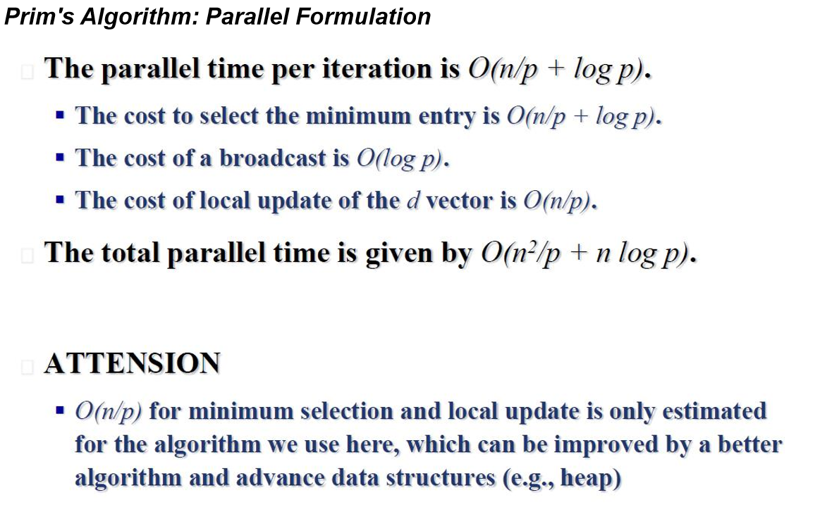
3. 单源最短路径 Dijkstra 的并行版本及复杂度。

4. 并行连接图算法原理。
- 跨进程划分图形,并在每个处理器上运行独立的连接组件算法。在这一点,我们有 p 个森林。
- 在第二步中,跨越森林两两合并,直到只剩下一个跨越森林。
- partition the graph across processes and run independent connected component algorithms on each processor. At this point, we have p spanning forests.
- In the second step, spanning forests are meged pairwise until only one spanning forest remains.
最小生成树算法
串行算法
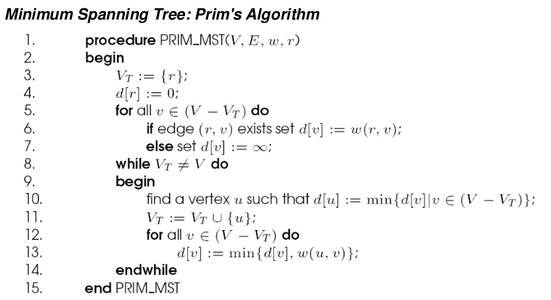
最小生成树(代价之和最小的生成树)
构造准则
- 尽可能用网络中权值最小的边
- 必须使用且仅使用 n-1 条边来联结网络中的 n 个顶点
- 不能使用产生回路的边。
普里姆(Prim)算法
算法流程
- 在连通网的顶点集合 V 中,任选一个顶点, 构成最小生成树的初始顶点集合 U;
- 在 U 和 V-U 中各选一个顶点,使得该边的权值最小,把该边加入到最小生成树的边集 TE 中, 同时将 V-U 中的该顶点并入到 U 中; 每次选择一个点未经过, 一个点经过, 避免了产生环.
- 反复执行第(2)步,直至 V-U=Ø 为止。
注意
- 若候选轻权边集中的轻权边不止一条,可任选其中的一条扩充到 T 中。
- 连通图的最小生成树不一定是唯一的,但它们的权相等。
实现
设置辅组数组 closedge[]
- lowcost 域:存放生成树顶点集合内顶点到生成树外各顶点的各边上的当前最小权值; U 集合 V-U 集合 3
- adjvex 域:记录生成树顶点集合外各顶点距离集合内哪个顶点最近(即权值最小)。
流程
- 初始化, 将 lowcost 初始化为$\infty$, adjvex 初始化为 0.
- 从 lowcost[v]$\neq$0 的点(选择一个属于 V-U 的点), 选择一个 lowcost[v]最小的顶点(如果全为$\infty$, 任选一个点作为出发点, 如果有点不为$\infty$, 此时选取到的点是 V-U 到 U 权值最小的边的点)
- 将 adjvex[v] 改为-1, 表示它已加入生成树顶点集合。
- 将边 (adjvex[v], v, lowcost[v] ) 加入生成树的边集合。
- 取
lowcost[i] = min{ lowcost[i], Edge[v][i] }, 即用生成树顶点集合外各顶点 i 到刚加入该集 合的新顶点 v 的距离Edge[v][i]与原来它们到 生成树顶点集合中顶点的最短距离 lowcost[i] 做比较, 取距离近的作为这些集合外顶点到生成树顶点集合内顶点的最短距离 - 如果生成树顶点集合外顶点 i 到刚加入 该集合的新顶点 v 的距离比原来它到生成树顶点集合中顶点的最短距离还要近, 则修改 adjvex[i] : adjvex[i] = v。表示生成树外顶点 i 到生成树内顶点 v 当前距离最近。
并行算法
- 外层的选点循环难并行
- 内层的循环容易并行
- 并行的地方是选取最近的点这一步
并行算法流程
- The adjacency matrix is partitioned in a 1-D block fashion, with distance vector d partitioned accordingly.
- In each step, a processor selects the locally closest node, followed by a global reduction to select globally closest node.
- This node is inserted into MST, and the choice broadcast to all processors. Each processor updates its part of the d vector locally.
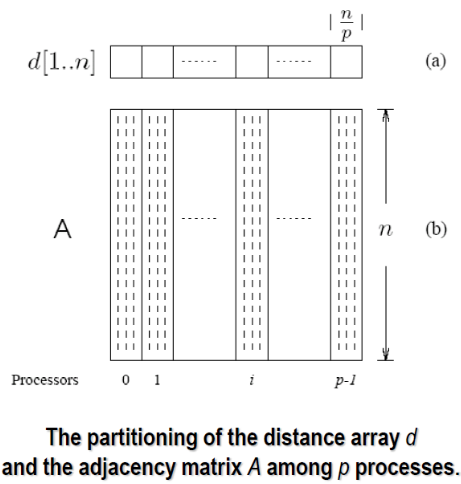
时间复杂度
并行算法每次迭代的时间复杂度为$O(n/p+logp)$
- 选取最近点$O(n/p+logp)$
- 广播$O(logp)$
- 本地更新距离矩阵$O(n/p)$
总时间复杂度为$O(n^2/p+nlogp)$
单源最短路径算法
最短路径(Shortest Path algorithms)
最短路径问题: 如果从图中某一顶点(称为源点)到达另一顶点(称为终点)的路径可能不止一条,如何找到一条路径使得沿此路径上各边上的权值总和达到最小。
问题解法
- 边上权值非负情形的单源最短路径问题 => Dijkstra 算法
- 所有顶点之间的最短路径 => Floyd 算法
Dijkstra 算法
本质上是贪心算法.
算法流程
- 初始化:
S ← { v 0 };dist[j] ← Edge[0][j], j = 1, 2, ..., n-1; - 求出最短路径的长度:
dist[k] ← min { dist[i] }, i in V- S;S ← S U { k }; - 修改:
dist[i] ← min{ dist[i], dist[k] + Edge[k][i] }, 对于每一个i in V- S; - 判断:若
S = V, 则算法结束,否则转 2。
并行版本
和 Prim 的优化非常近似, 分析和完全考虑 Prim 的并行版本
All-pairs 最短路径算法
Dijkstra
使用的话, 复杂度为$O(n^3)$, 并行化有两种方法
- (source partitioned) execute each of the n shortest path problems on a different processor
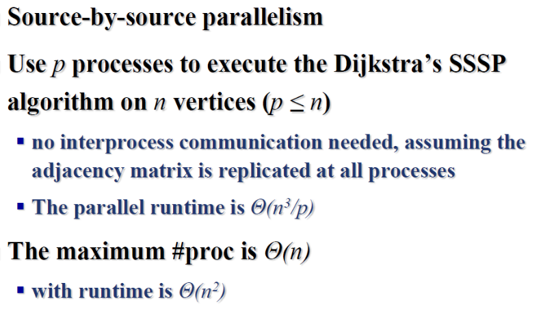
- (source parallel) use a parallel formulation of the shortest path problem to increase concurrency
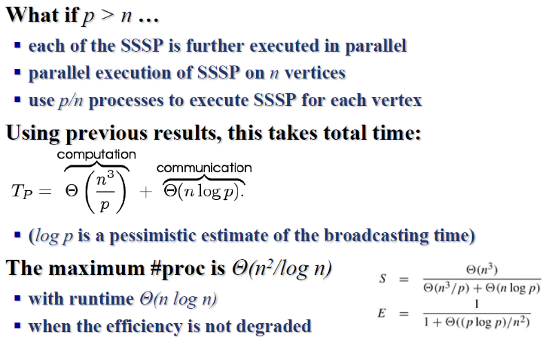
Floyd’s Algorithm
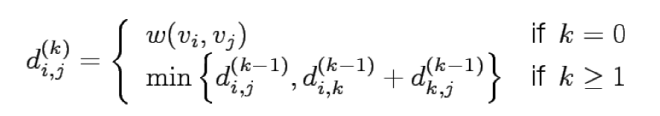
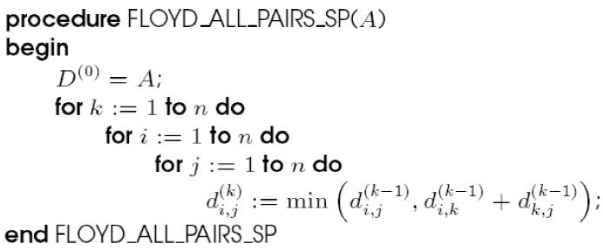
Floyd’s Algorithm (1-D Block Mapping)
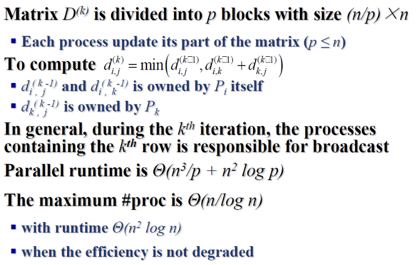
Floyd’s Algorithm (2-D Block Mapping)
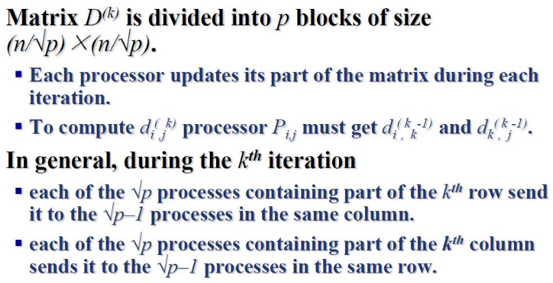
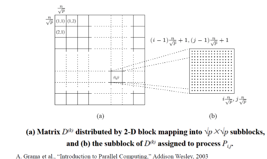

Floyd’s Algorithm: Communications

Connected Components
可以使用 DFS 寻找图的连通分量
并行化可以使图在不同的处理器上运行不同生成树 DFS, 最后再合并.
Related posts